Logic gates, also known as logical connectives, represent a set of Boolean operations that take in a set number of inputs, which is know as its arity. Within the context of computer architecture, logical connectives lie at the center point of the industry, enabling digital logic engineers to craft complex systems capable of computation out of simple connectives. Furthermore, within highly transistor efficient computer architectures, the connectives often manifest as “functionally complete,” meaning that the connective can create all other possible connectives solely through compositions with itself. Post’s Functional Completeness Theorem helps narrow down the conditions required for a connective to be functionally complete. The Formula For the Number of Sheffer Functions helps specify the number of functionally complete gates there are of a given arity. Using these two notions, I investigate the conditions in which a connective may appear to be functionally complete, and computationally derive the expressions of all other gates as compositions of a functionally complete one. I then expand this definition to emulate logic/rule-based systems of cellular automata.
Introduction
Introduction
Cellular automata are a pattern generated by a set of rules, indicating whether a given cell of a graph will live onto the next generation. Cellular automata (CA) have been used to model population growth, fire spreads, and partial differential equations. There are many different ways in which the rules can manifest. CAs such as Rule 110 and Conway’s Game of Life have rules that are dependent on the presence of other cells. Mathematically, rules are logical expressions.
Cellular automata offer a visual understanding of what a logical operation does to an initial state. When CA produces eccentric and visually interesting patterns, the process of generating such a pattern is often obscured. After understanding how to backtrack to a rule, a natural extension is to understand how gates of an arity can make up other gates, which may result in more complex rules. This is the notion of functional completeness, which I will expand on later in this essay.
Cellular automata offer a visual understanding of what a logical operation does to an initial state. When CA produces eccentric and visually interesting patterns, the process of generating such a pattern is often obscured. After understanding how to backtrack to a rule, a natural extension is to understand how gates of an arity can make up other gates, which may result in more complex rules. This is the notion of functional completeness, which I will expand on later in this essay.
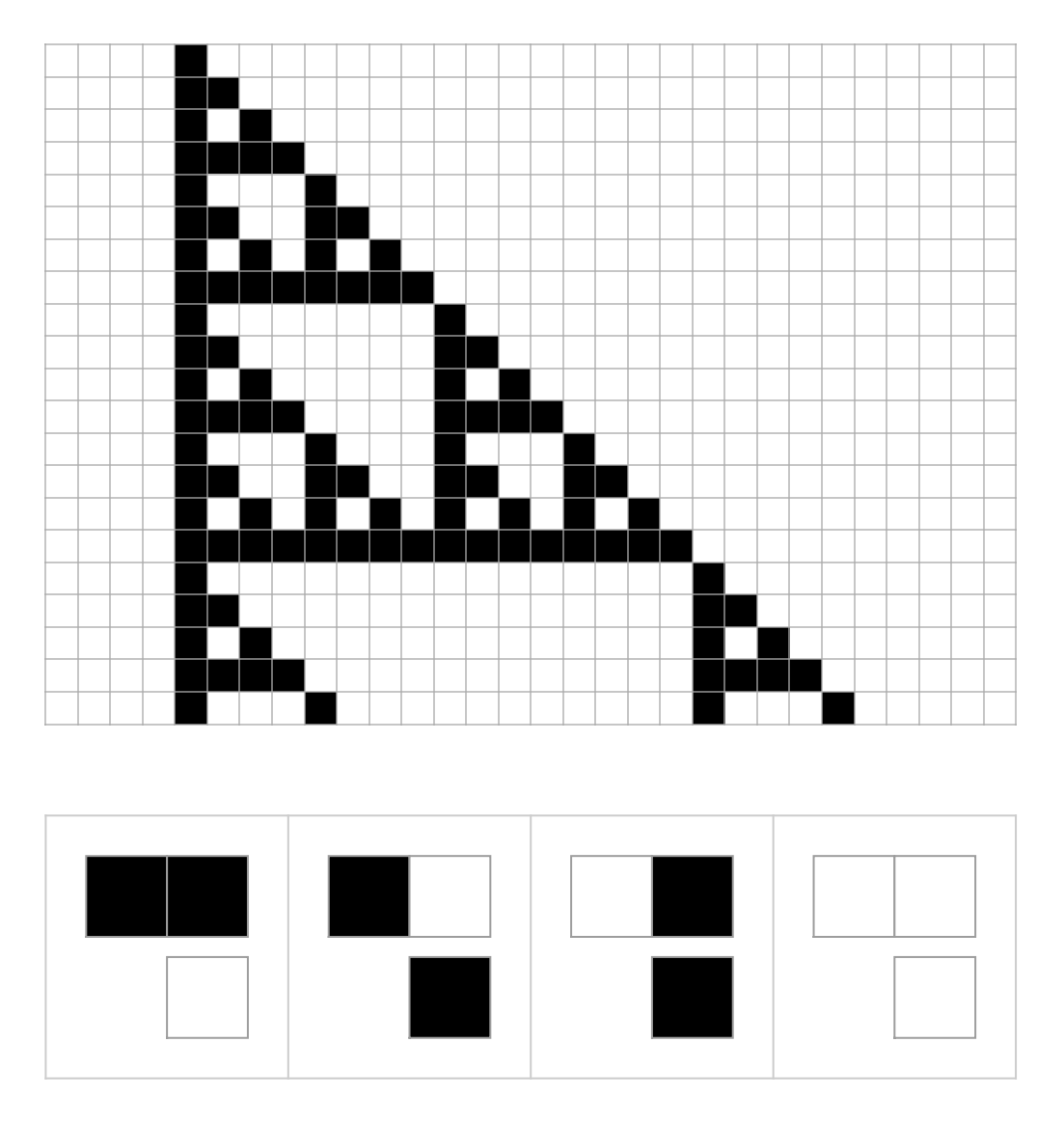
An automata with XOR as a rule, with a following rule plot, or truth table, displaying a self similar pattern:
In[]:=
GraphicsGridArrayPlotCellularAutomaton[{6,2,1/2},{CenterArray[1,10],0},{20,All}],,RulePlotCellularAutomaton[{6,2,1/2}],
Out[]=
Exhaustively Finding the Rule of a 2:1 Cellular Automaton
Exhaustively Finding the Rule of a 2:1 Cellular Automaton
Now this is a square cellular automata governed by a logical expression as a rule. In this specific scenario, the rule is XOR(p, q) for Booleans p, q. The reason I made a custom one and didn’t make use of the in built CellularAutomaton function is because I wanted to specify the input as a Boolean function. The function is iterative, using NestList to find the pattern for future generations.
Defines how to create the next row given a given a previous rule:
In[]:=
nextRow[rule_,offsets_:{1,0}][row_List]:=MapThread[rule,RotateLeft[row,#]&/@offsets];
Specify a Boolean automaton function that can be repeated for a certain number of generations, with the ability to specify an offset on what cell to generate
In[]:=
booleanAutomaton[rule_,initialRow_List,steps_Integer,offsets_:{1,0}]:=NestList[nextRow[rule,offsets],initialRow,steps];
Initialize a random initial state for the CA to begin with:
In[]:=
randomInitialRow[width_Integer?Positive]:=RandomChoice[{True,False},width];
Display the automaton on a grid with a mesh:
displayAutomaton[grid_List]:=ArrayPlotBoole[grid],;
Import the resource function “TruthTable” to visualize truth tables of logical connectives:
In[]:=
truthTable=ResourceFunction["TruthTable"];
Truth table of XOR for reference:
In[]:=
truthTable[Xor[a,b],{a,b}]
Out[]=
a | b | a⊻b |
True | True | False |
True | False | True |
False | True | True |
False | False | False |
This is offset here, the first input is the top left and the other is the center to produce a cell under the center.
Define the rule that will be used as well as the output grid to display:
rule=Function[{a,b},Xor[a,b]];displayAutomaton[booleanAutomaton[rule,randomInitialRow[25],25,{-1,0}]]
Out[]=
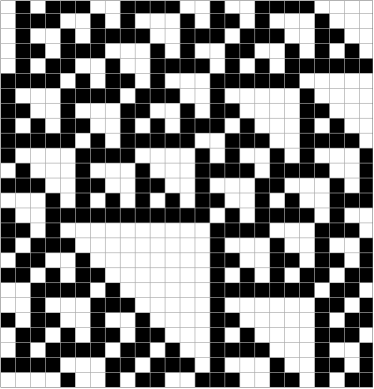
I’ve got a cellular automaton based on some logic function (XOR, rule 6) here. The first row is randomized and one can see the development of the pattern. The cellular automaton can also be backtracked to decipher the rule that generated it. For example, one would need to find each possible input combination next to each other and map that Boolean output to a truth table. Since I’m are only using gates of arity 2, there is a high chance that I can find all of the possible input conditions within our grid. Similarly, this is easier for 2:1 Boolean logic rules because there are only 16 possible logic gates of arity 2.
()
2
2
2
To identify the rule of this automaton, one can find all the input conditions. I could take all the input conditions and create an association to define a rule.
The Shortcomings of An Exhaustive Approach
The Shortcomings of An Exhaustive Approach
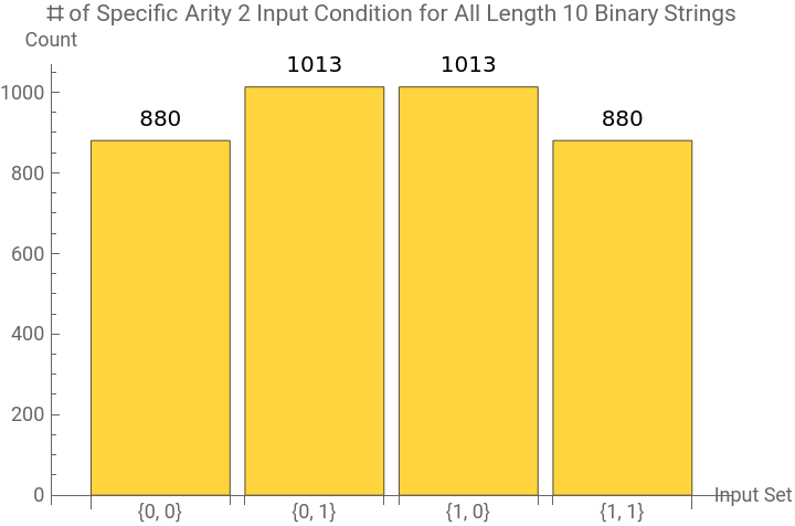
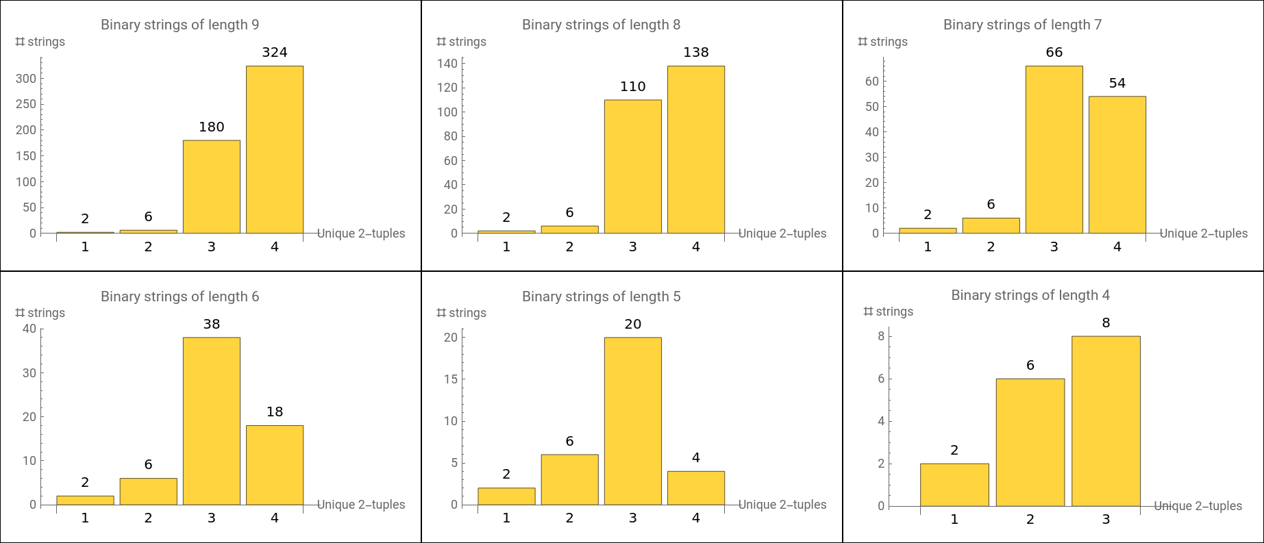
For all possible length 10 binary strings, we can find the below distribution of each of the any length 2 binary tuple. Since there are less instances of {1,1} and {0,0}, there must be some binary string of length 10 that cannot be solved when analyzed via the brute force method that I described for classical 2:1 gates. In fact, as the initial state for the cellular automata decreases in length (i.e. the row shrinks in size), the amount of strings that have all 4, length 2 binary string tuples decreases.
Bar chart showing the amount of each possible length 2 binary input occurs within all tuples of length 10:
In[]:=
BarChartDataset[AssociationThread[Tuples[{0,1},2]->Table[Count[Tuples[{0,1},10],str_/;MemberQ[Partition[str,2,1],tuple]],{tuple,Tuples[{0,1},2]}]]],,
Out[]=
Plot displaying the count of how many length 10 binary strings contain a certain amount of the total possible amount of binary inputs:
In[]:=
BarChartDataset[Counts[Length[DeleteDuplicates[Partition[#,2,1]]]&/@Tuples[{0,1},10]]],,
Out[]=
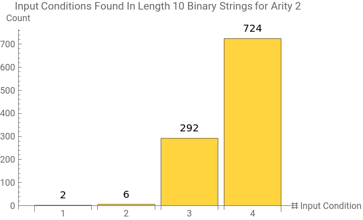
For initial binary string of length 10, there are 724 possible configurations that contain all 4 of the possible inputs. Therefore, the brute force method would apply to those types of strings. However, this is not generalizable to all initial states. As the length of the initial row decreases, there are less combinations that contain all 4 strings. Eventually, once the size of the initial state is length 4 or below, it becomes impossible for all 4 input conditions to coexist.
Grid of a number of plots showing how it becomes more difficult to find all possible input conditions as the size of the initial conditions decrease:
In[]:=
createChart[length_]:=With{counts=Counts[Length[DeleteDuplicates[Partition[#,2,1]]]&/@Tuples[{0,1},length]]},BarChartKeySort[counts],ChartLabelsPlaced[Keys[KeySort[counts]],Below],
In[]:=
GraphicsGridPartition[Table[createChart[length],{length,9,4,-1}],3],
Out[]=
Finding a Functionally Complete Gate
Finding a Functionally Complete Gate
Checking With Post’s Functional Completeness Theorem
Checking With Post’s Functional Completeness Theorem
A function is denoted functionally complete if it fails to exhibit all 5 of these conditions.
1
.Preserving 0: if all inputs are 0, the output must be 0
2
.Preserving 1: if all inputs are 1, the output must be 1
3
.Linearity: inverting an input either always changes the output or never does
4
.Monotonicity: increasing the inputs (0→1) must never make the output decrease(1→0)
5
.Self-Duality: if all the inputs are inverted, the output should also be inverted
Why NAND is Functionally Complete
Why NAND is Functionally Complete
Consider NAND, a functionally complete gate. The truth table of a 2:1 NAND gate is:
Truth table for a 2 input NAND gate for reference:
NAND aptly fails all 5 of Post’s conditions.
◼
When the input is (0,0), the output is 1. So NAND fails this condition.
2
.Preserving 1:
◼
When the input is (1,1), the output is 0. So NAND fails this condition.
3
.Linearity
◼
When the input is (1,1), the output is 0. However, when the input is (1,0), the output is 1. But, when the input is (0,1), the output is also 1. So NAND fails this condition.
4
.Monotonicity
◼
When the inputs go from (0,0) to (1,1), the output decreases from 1 to 0. So NAND fails this condition.
5
.Self-Duality
◼
When the inputs are changed from (1,0) to (0,1) via bitwise inversion, the output does not change. So NAND fails this condition.
An Important Equation
An Important Equation
Filters for failures in Post’s conditions for all length 8 binary strings, explicitly checking preserving and linearity rules:
Find all functionally complete gates of arity 3:
Convert all of the functionally complete truth tables into a rule for a cellular automata:
The following cellular automata are made up of functionally complete rules. Since each of these are each 3:1, they can even be composed within themselves in some manner to produce the famous, Turing-complete, Rule 110!
All 56 functionally complete cellular automata expressed aged 20 generations from a common initial position:
Rule 110 for reference, any of the above automatons can generate this via composition alone:
Defining How To Compose Functions
Defining How To Compose Functions
To find all of the possible compositions, I employed a recursive function to find all of the open spots within a function of a set arity and replace each input with another function depending on a specified depth. This is a brute force approach of finding all of the possible compositions of functions. At first, there was difficulty in computing, but after employing a couple of tricks, I drastically improved the computation speed by vastly reducing the space at which the function has to recurse. This function works by establishing a basis of 3 variables, and then repeatedly placing each of them in all combinations within the a specified function. This approach rapidly increases the space of all compositions that I am keeping track of.
Load in the InverseBoole resource function for ease of use:
Creates an association between the inputs and outputs of a logic gate:
Recursive algorithm to find all compositions of a truth table with itself:
Recursive algorithm to find all compositions of a truth table with itself (for binary... less computationally expensive):
Finding Compositions
Finding Compositions
Test With Arity n = 2
Test With Arity n = 2
To be able to find the most “reduced” functional expression, I need an algorithm that finds all of the compositions of a function of a given arity and checks all of the unique truth tables that they produce. I will start by creating some helper functions, and then move onto applying this to gates of arity 2. It is known that the 2 functionally complete connectives of arity 2 are NAND and NOR.
Confirming that our checks with Post’s Theorem finds NAND and NOR as functionally complete. Each of these are the DeMorganized outputs of NAND and NOR:
Create a logical association between all inputs and defined outputs:
NAND has been exhaustively shown to be functionally complete using our function! Since it returns all 16 possible truth table outputs for arity 2, all possible 2:1 functions can be modeled by NAND.
Shows all truth tables that a given truth table, in this case {1, 1, 1, 0} (aka NAND) can create from compositions with itself:
This is a similar case for NOR. Like NAND, it also returns all 16 logic gates which proves that it’s functionally complete.
Shows all truth tables that a given truth table, in this case {1, 0, 0, 0} (aka NOR) can create from compositions with itself:
Creates a grid of all the compositions of NOR with itself to produce every arity 2 logic gate in increasing binary order from left to right:
Creates a grid of all the compositions of NAND with itself to produce every arity 2 logic gate in increasing binary order from left to right:
People often hear that NAND is a more “efficient” gate than NOR. In fact, within computer engineering, it is, but within the lens of functional completeness, they perform quite similarly. I’m measuring efficiency by the depth needed to generate a logic gate. This is because there is more computation involved to reach find the output of a logic gate that has many nested gates within itself. The mean depth required to generate all 16 connectives for arity 2 are the same. However, I’ll define a tiebreaker as the connective that has less higher depth gates.
NOR appears to have less depth 3 connectives than NAND, so therefore it would mean that it is more “efficient”:
NOR appears to have less depth 3 connectives than NAND, so therefore it would mean that it is more “efficient”:
All 2:1 gates in terms of f=NAND displayed as tree graphs:
Expansion to Arity n = 3
Expansion to Arity n = 3
This recursive composition approach is effective but hits a couple of roadblocks. For NAND, it is only able to generate 250 of the tuples, meaning it overlooks 6 tuples that are important. My theory is that there are a couple of gates that have depth 4. Also, for “efficient” gates (ex: the one Christopher Wolfram showed), since there are more gates that match unique truth tables found in depth 2. This means that the space that depth 3 and 4 needs to search is much larger, rapidly increasing the number of combination that the algorithm needs to search for.
Converts a functional expression into a truth table:
Deletes the duplicate elements that are present in a generated set of expressions:
Creates an association between the possible inputs and outputs of a function:
Creates a truth table based on a functional term, specifying NAND as a rule:
Find all depth 2, 3:1 gates. Note, this can take several minutes:
Collect all equivalent terms into their own class, since many of the compositions are redundant and equivalent when evaluated:
Collect the first element of each equivalence class, because that’s the most efficient functionally expression (least depth):
The algorithm to place expressions in every argument position of expressions of higher depth:
Repeat the process of increasing the depth of the expressions that was already derived in testSet (very narrowed down functional space):
Again, gather the newly generated terms into their own equivalence class:
Again, take the first expression of each equivalence class and compile into a final list:
Oh no! There’s only 250 and not 256:
Finds the length of all the expressions that were found
An Alternative Approach To Nested Compositions
An Alternative Approach To Nested Compositions
Since the previous approach to finding the compositions did not suffice, I’ll have to adopt a more rigorous approach. This approach directly composes truth tables within itself to generate a new truth table, and then checks if that truth table is novel. Repeating this over time, means that it should output 256 compositions, regardless of their efficiency due to FixedPoint. I got all 256 compositions here.
Converts a truth table to a binary string:
Composes 3 truth tables within itself to get a resultant connective:
The initial terms that helps initiate the composition process:
Creates an association between the terms and the truth tables, for easier navigation later:
Generates new terms using the compostTermTriple function:
Adds the new association to a growing term list:
Continuously add new terms, growing from the initial terms until it is no longer possible to make more connectives (limit is 256 for arity 3):
The function compositions for 3:1 NAND, which have previously shown to be functionally complete. Note: this can take several minutes:
Organize the functional expressions that were derived:
It is impractical to create a tree of all 256 compositions, but I’ll show an animation of all of them that may suffice. The animation increases in binary order and shows all 256 gates of arity 3 expressed as a logical connective.
Creates an animated list of functional trees of all 256 arity 3 connectives, purely composed with g=NAND of arity 3 rendering at 3 FPS:
Conclusion
Conclusion
This methodology is effective at generating many of the functionally complete gates of some arity. In practice, connectives with high arities, which I’ll estimate to be greater than 5, are ineffective due to lack of power. However, extended arities and functional completeness offer promising results to emulate logic components such as multiplexers. From the aspect of cellular automata, finding a even “simpler” rule than an already established rule is an exiting premise to think about. It’s fascinating to understand why simple logic gates like NAND and NOR are able to create such intricate technologies, and their functional completeness is foundational in creating all sorts of processors etc.
Future Directions
Future Directions
Acknowledgements
Acknowledgements
I would like to extend heartfelt thanks to my mentor Adam Millar for his immense support throughout this project. His guidance and vast expertise in logic made the research process streamlined, and I learned a lot from his conversations and explanations. Additionally, I would like to thank Dugan Hammock for his extended interest my project and help with programming in Wolfram Language. I would also like to extend my gratitude to the program directors, Eryn, Rory, Megan, and Cyrus for their commendable organizational skills and support through the program.
Additional thanks to Stephen Wolfram for suggesting this project. Lastly, I would like thank my TA group and TA for making this program experience unforgettable. I’m glad that I was able to connect with a large group of amazing people.
References
References
1
.Maksimović, P., & Janičić, P. (2006). Simple characterization of functionally complete one-element sets of propositional connectives. https://poincare.matf.bg.ac.rs/~janicic//papers/2006-mlq-complete-sets.pdf
2
.Pelletier, F. J., & Martin, N. M. (1990). Post’s functional completeness theorem. Notre Dame Journal of Formal Logic, 31(2), 462–475. https://projecteuclid.org/journals/notre-dame-journal-of-formal-logic/volume-31/issue-3/Posts-functional-completeness-theorem/10.1305/ndjfl/1093635508.pdf
3
.Wolfram, S. (2024, August 22). What’s really going on in machine learning? Some minimal models. Stephen Wolfram Writings. https://writings.stephenwolfram.com/2024/08/whats-really-going-on-in-machine-learning-some-minimal-models/
4
.Wolfram, C. (2016). Functional Completeness and Optimization. christopherwolfram.com. https://christopherwolfram.com/projects/functional-completeness/
CITE THIS NOTEBOOK
CITE THIS NOTEBOOK
Functional completeness among logic gates of arity N
by Samarth Bhat
Wolfram Community, STAFF PICKS, July 9, 2026
https://community.wolfram.com/groups/-/m/t/3752491
by Samarth Bhat
Wolfram Community, STAFF PICKS, July 9, 2026
https://community.wolfram.com/groups/-/m/t/3752491