Dolphin communication has always been a blackbox of marine life, where deciphering their linguistic code could revolutionize our understanding of non-human intelligence and reshape marine conservation efforts. This computational essay introduces a method for translating raw hydrophone recordings of Tursiops (more commonly known as bottlenose dolphins) into a lexicon of “phonemes”. By analysing the features of each possible sound unit across numerous dolphin whistle audios, patterns of recurring sequences are discovered and clustered into their respective set of vectors based on their audio features. Thus the first inventory of dolphin phonemes was created by inventing symbols corresponding to each set of respective characteristics. These symbols can then be applied back onto any set of dolphin audio to detect which sequence of phonemes could be linked together and function like words. Instead of relying on potentially unreliable heavy machine-learning models, this research relies on transparent signal analysis, thereby offering a clear method that contributes towards bio-acoustic linguistics research.
Introduction
Introduction
Dolphins have the second-highest encephalization quotient (the ratio of brain size to body size) after humans and are widely considered to be one of the most intelligent animals on earth with their advanced cognitive abilities and intricate social structures. Studies have repeatedly shown that they exchange information during cooperative problem-solving and conflict resolution—from synchronizing bubble-net hunts to coordinating calf care—yet the internal logic of their acoustic “speech” remains a mystery. Past research confirms that dolphins utilize whistles, clicks, and burst-pulse sounds for individual identification, social bonding, task coordination, and emotional expression. But one question remains: Do dolphins use meaningful, human-like phonemes as the foundation of their vocal system?
This study takes a practical approach toward decoding dolphin whistles. While there has been no prior research or definition of dolphin phonemes, a dolphin phoneme, as used here, is defined as the smallest distinct frequency contour that seems to carry consistent features, much like human language. The dataset for the audios used in this research project was acquired from IEEE DataPort, where over 3000 bottlenose dolphin whistles were manually identified and extracted by passive-acoustic-monitoring experts from over 24 hours of recordings. Instead of starting with the entire raw dataset recordings, we begin our analysis on a single whistle-cleaning, segmenting and extracting its features—before scaling the procedure to all recordings to find recurring motifs that are later assigned as symbols.
This study takes a practical approach toward decoding dolphin whistles. While there has been no prior research or definition of dolphin phonemes, a dolphin phoneme, as used here, is defined as the smallest distinct frequency contour that seems to carry consistent features, much like human language. The dataset for the audios used in this research project was acquired from IEEE DataPort, where over 3000 bottlenose dolphin whistles were manually identified and extracted by passive-acoustic-monitoring experts from over 24 hours of recordings. Instead of starting with the entire raw dataset recordings, we begin our analysis on a single whistle-cleaning, segmenting and extracting its features—before scaling the procedure to all recordings to find recurring motifs that are later assigned as symbols.
Importing Data from IEEE
Importing Data from IEEE
Once we have the whistle signal zip file downloaded onto the computational device, we can attach the file path onto the series of functions below in order to import the isolated audio of all the whistles.
whistleSignalsMaster="(*File Path to IEEE Whistle_Signals Folder*)";whistleSignalFolderNames=FileNames[All,whistleSignalsMaster];whistleSignalFileNames=(FileNames[All,#]&/@whistleSignalFolderNames)//Flatten;iEEEWhistles=Import[#,"Audio"]&/@whistleSignalFileNames;
Whistle filter
Whistle filter
Removing background noise such as water and engine rumble are crucial to acquiring accurate data and features from the whistle audio. The typical range of frequency for the whistles of a Bottlenose dolphin is ~4kHz-22kHz (Marley et al. (2017)). Therefore, after benchmarking several filter function and frequency cutoff pairs, a band-pass filter fine-tuned to that range was ultimately chosen, as it produces the best result and offered the cleanest spectra.
Raw dolphin whistle audio example (We will be using whistle 16 for all our tests).
In[]:=
iEEE16=iEEEWhistles[[16]];
Filtered dolphin whistle audio.
In[]:=
iEEE16B=BandpassFilteriEEE16,,;
Open access example of dolphin whistle audio.
In[]:=
publicIEEE16Whistle=CloudPut[iEEE16];CloudObject[publicIEEE16Whistle,Permissions->"Public"];SetPermissions[publicIEEE16Whistle,"Public"];CloudGet[publicIEEE16Whistle]
Out[]=
Open access example of filtered dolphin whistle audio.
In[]:=
publicIEEE16FilteredWhistle=CloudPut[iEEE16B];CloudObject[publicIEEE16FilteredWhistle,Permissions->"Public"];SetPermissions[publicIEEE16FilteredWhistle,"Public"];CloudGet[publicIEEE16FilteredWhistle]
Out[]=
Time frequency plots
Time frequency plots
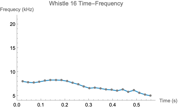
For visualization purposes, we can use various graphs to ensure the frequency contour detected from the filtered audio matches up with the spectrogram.
In[]:=
Spectrogram[iEEE16B]
Out[]=
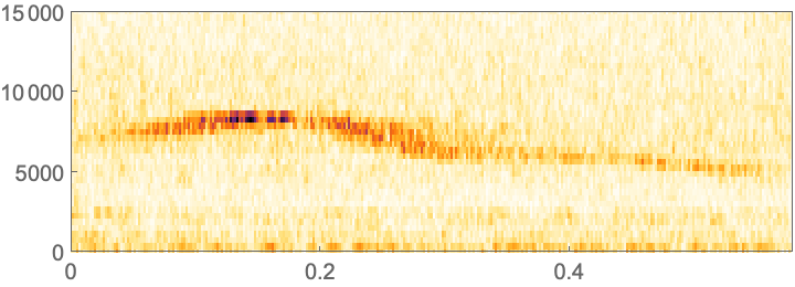
Continuous ListLinePlot that matches the recognized pitches of the whistle audio.
In[]:=
ListLinePlotPitchRecognizeiEEE16B,AllowedFrequencyRange->,,AcceptanceThreshold->.51000,PlotRange->{{0,Duration[iEEE16B,None]},{4,21.907}},PlotLabel"Whistle 16 Time-Frequency",AxesLabel->{"Time (s)","Frequecy (kHz)"},Mesh->Full,MeshStyle{PointSize[Medium],Gray}
Out[]=
Create into Functions through Interpolation
Create into Functions through Interpolation
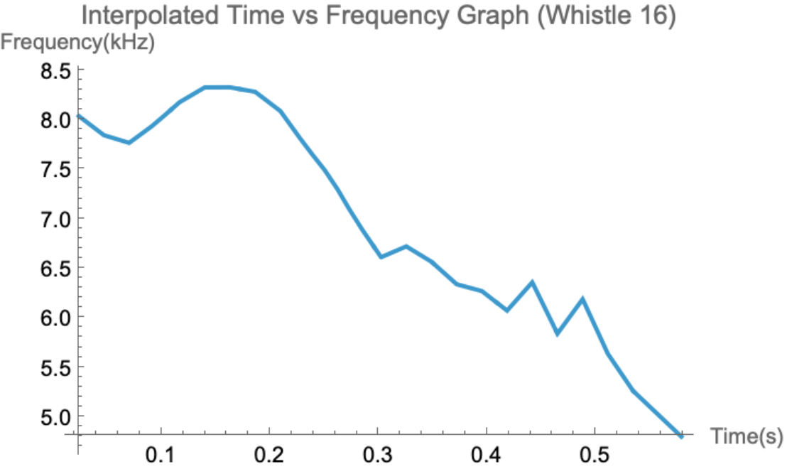
Next, we have to convert the recognized frequency points into an actual function in which we can extract specific data points/characteristics from the audio. This will then yield a continuous whistle contour from which the time interval, zero-crossings, and other boundary cues for phoneme segmentation can be extracted with millisecond precision.
If a whistle has missing values in the beginning (a period of silence before the dolphin whistle within the audio recording), the function will return an extrapolation error message saying that an input value lies outside the range of data in the interpolating function, resulting in a bizarre output when trying to find the Min or Max extrema. To fix this problem, we have to add DeleteMissing around the lacking frequency time points, which outputs the precise timeseries.
In[]:=
pitchData1=DeleteMissing[PitchRecognize[iEEE16B,AllowedFrequencyRange->{4000,21907},AcceptanceThreshold->.5]/1000];
Since PitchRecognize recognizes the frequency of an audio in hertz, we need to remove the units from the list of time-frequency data points.
In[]:=
listNoMagnitude=Table[{First@point,QuantityMagnitude@Last@point},{point,pitchData1["Path"]}];
In[]:=
int=Interpolation[listNoMagnitude,InterpolationOrder->1];
In[]:=
{tMin,tMax}=int["Domain"][[1]];
Below is the graph of the interpolating function, where the range of the x-axis set to the beginning and end of the whistle range.
In[]:=
functionPlot=Plot[int[x],{x,tMin,Duration[iEEE16B,None]},PlotLabel"Interpolated Time vs Frequency Graph (Whistle 16)",AxesLabel{"Time(s)","Frequency(kHz)"}]
Out[]=
Finding the Derivative
Finding the Derivative
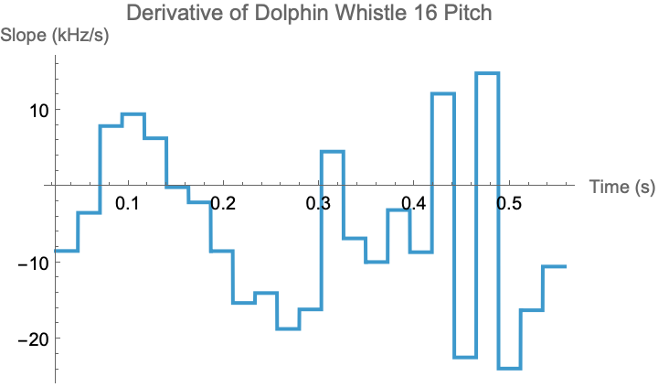
The derivative of the interpolated function records whether the instantaneous pitch is rising (positive) or falling (negative). Every zero-crossing (sign change) marks a local extremum and thus a natural boundary between pitch sweeps. By splitting the whistle into segments at each change in pitch direction, we can extract the time intervals of each segment in the whistle. Afterwards, we take the derivativeValues of the interpolated whistle contour function which essentially reveals the structure and boundaries within the whistle, thereby segmenting the whistle into meaningful chunks that likely correspond to different “phoneme-like” units in dolphin communication.
The first line is the function for the original whistle contour, while the second is the function for its derivative (the slope or “change” at each point in time).
In[]:=
ogWhistle[x_]:=int[x]ogWhistlePrime=int';
The derivative graph plot below aids in visualizing when the derivative = 0, which will help in the next step of segmentation.
In[]:=
ogWhistlePrimeFunc[x_]:=QuantityMagnitude[ogWhistlePrime[x]]Plot[ogWhistlePrimeFunc[x],{x,tMin,tMax},AxesLabel->{"Time (s)","Slope (kHz/s)"},PlotLabel->"Derivative of Dolphin Whistle 16 Pitch"]
Out[]=
Extracting segments from one zero cutting to the next
Extracting segments from one zero cutting to the next
Now that we have the derivative of the interpolated function, we can extract the list of derivative values for the whistle and capture how the whistle pitch is changing over time.
In[]:=
dt=0.001;sampleTimes=Range[tMin,tMax,dt];derivativeValues=ogWhistlePrime/@sampleTimes;
First, we pair consecutive derivative values to look for points where the sign changes, then we select the pairs where the derivative sign flips (zero-crossings), and finally calculate the mean time for each zero-crossing to estimate the precise boundary and get the time intervals for each detected segment.
In[]:=
derivativePairs=Partition[Transpose[{sampleTimes,derivativeValues}],2,1];signChangePairs=Select[derivativePairs,(#[[1,2]]*#[[2,2]]<0)&];zeroCrossingTimes=Mean/@(signChangePairs[[All,All,1]]);allBoundaries=Join[{tMin},zeroCrossingTimes,{tMax}];segments=Partition[allBoundaries,2,1]
Rescale
Rescale
For phoneme-like analysis, we need to be able to extract the features from each segment into vectors in order to be able to compare each whistle systematically. Therefore we have to rescale the x-axis (time) to a standard unit interval, [0,1] in this case, and sample it at a fixed resolution (e.g. 50 equally spaced points). This normalization removes absolute-duration bias and allows other frequency contour descriptors such as slope, mean, and range to be compared directly across phoneme candidates.
Rescaled example of the list of frequencies points over the first time interval/segment.
Visualizing the features of Whistle 16
Visualizing the features of Whistle 16
Compared to the full frequency-time graph of whistle 16 defined as functionPlot above, the graphs below clearly illustrates how the sample whistle is subdivided and rescaled to easily compare between segments.
The graph of each segment in the sample whistle audio side by side.
All the segments in the sample whistle audio overlaid onto one graph.
Initial Feature Extraction
Initial Feature Extraction
We have to extract comparable features within each segment into the categories below. While we considered curvature (a shape descriptor of a segment that reflects its complexity of movement over time—the higher the curvature, the more modulated and complex the whistle’s frequency shape is; the lower the curvature, the simpler and flatter the segment), the actual duration of each segment, and standard deviation, I ultimately decided to just evaluate the three most important features: slope, mean, and range of the frequency.
Although a six-dimensional feature vector (slope, mean, range, curvature, duration, standard deviation) looks richer than the three-dimensional one, it introduces two main problems:
1. Loss of interpretability
With more than three axes we can no longer inspect the raw feature space directly; Wolfram’s FeatureSpacePlot3D silently projects the data down (often via internal PCA), stripping away axis labels and hiding which original attributes drive the grouping. This opacity makes it hard to diagnose misgroupings or to map clusters back to meaningful acoustic traits.
2. Dimensionality & complications in clustering
In high-dimensional spaces distance metrics flatten out: points tend to look equally far apart, making algorithms and clustering unstable. For example, insignificant curvature and standard-deviation values occasionally caused segments that clearly ought to be neighbors to drift apart, while unrelated segments collapse into the same centroid. The result is a dendrogram with shallow merge heights, a silhouette score that hovers near zero, and plots that reshuffle every time you nudge a parameter.
These complications can also be seen below. Therefore concentrating only on slope, mean, and range maximises discriminative power while keeping the clustering stage transparent, offering tighter clusters that are easy to validate and to relate back to real dolphin acoustic behaviour.
All 6 vectors of whistle 16 in a 3D plot.
A 3D plot extracting 3 vectors (slope, mean, and range) of each segment in the sample whistle 16 with clear and interpretable axes labels.
Generalized Feature Extraction for Each Segment of Whistles
Generalized Feature Extraction for Each Segment of Whistles
The module function below takes in a single dolphin whistle audio clip and applies a series of functions that allow us to compare each possible phoneme. Like the process described above, the code below is a generalized version carrying out essentially the same procedures. We first preprocess the audio by filtering the background/water/engine noises, then transform it into a list of time-frequency points, which is interpolated into a continuous time-frequency function, followed by defining segments based on the interval between each zero-crossings in the derivative of the pitch contour. Finally, each segment is analyzed for a set of descriptive features (slope, curvature, and frequency range), allowing for consistent comparison and clustering of segments across different whistles.
Each segment is rescaled in time to a 0-1 range which helps isolate each possible phoneme for comparison and clustering.
Calculate the 3 most significant vectors: slope, mean and range of each segment’s frequency.
This getData function is a generalised and cleaned version of the process described above—essentially segmenting and extracting all 3 feature vectors (slope, mean, range) for any/all dolphin audio.
Generating a list of features (slope, mean, range) of every single segment in all the Bottlenose dolphin audio clips from IEEE.
Ensuring the features are in the correct format: Multiple lists of sublists.
After applying the getData function onto every dolphin whistle audio from IEEE, we found 29899 total segments!
Evaluating automatic clustering and visualization methods
Evaluating automatic clustering and visualization methods
Beyond the workflow documented in this computational essay, I experimented with a plethora of clustering methods and projections such as TSNE, Latent Semantic Analysis, Principal Component Analysis, UMAP as well as an assortment of 2-D and 3-D scatter visualisations. Throughout this “dolphin detective” process, many of the plots appeared visually striking, yet the latent axes offered no clear acoustic interpretation, nor did the data points seem to hold any form of significant meaning which we could effectively analyse and interpret. Finally, after countless computer crashes and errors, I came to the conclusion of the clustering method I would use—below is an illustrative example of how I approached this problem.
This code clusters the list of feature vectors into groups with similar characteristics using Wolfram’s default automatic clustering algorithm.
We export this file to save this large amount of data onto a computer in case the more sophisticated clustering in the following steps causes a crash.
A 3D scatter plot of the first 10,000 feature vectors from all clusters, plotted by their main features with FeatureSpacePlot3D.
We have to take the first part of notScaledClusterwithoutCSDD because we are focusing on the feature vectors that belong to a specific cluster, which preserves the meaningful groupings produced by the clustering algorithm. If we were to simply flatten notScaledClusterwithoutCSDD and plot it as above, it would mix together all the feature vectors from different clusters, losing their cluster assignments and resulting in an inaccurate plot.
While the clusters on this test graph is fundamentally what we are looking for, one obstacle was that unlike FindClusters, FeatureSpacePlot3D isn’t meant to be used as a clustering tool. The groupings exhibited look promising at first, but they are not true clusters—it’s more so just plotting with selected features and any apparent groupings are just a side effect of that. This is not ideal as we want to find out the mean characteristics of each of these clusters in order to be able to assign possible symbolic phonemes to them.
Clustering Method
Clustering Method
In order to find tangible values within each cluster, we have to extract the coordinates from the cluster plot, match each cluster to the corresponding data value in iconized3FeatureCluster, then finally run a clustering algorithm on the coordinates from FeatureSpacePlot3D (instead of on the data itself) so that we can identify the groupings apparent in FeatureSpacePlot3D. Although this method may produce a cluster count that is more/less than expected, we can fine-tune FindClusters by adjusting its parameters to discard any stray or insignificant clusters.
In theory, one would strive to run all 29175 segment feature vectors; however, due to a limitation in computational power, the max amount of data I was able to run was 12500. Nevertheless, the results found were still significant enough for analyzing the overall clustering patterns and should be considered valid.
This series of code clusters the original data by their standardized features and reconstructs the original grouped data for further analysis.
Visualization of the initial clustering of the 12500 segments without applying any parameters.
This detects how many rudimentary clusters there are in the data (in this case, 12500 segments).
Refinement for final clusters
Refinement for final clusters
Intuition tells us that there are probably not 112 individual whistle phonemes that a dolphin can produce. Additionally, as we can see below, there are a handful of clusters that have relatively insignificant amounts of segments assigned to them. These smaller groups could either be glitches at the edges of the recording, residual engine noises, or the occasional burstpulses, clicks, or squeaks that bottlenose dolphins can emit. These noises can warp a segment’s slope and range just enough to isolate it and should not be accidentally classified as stable phonemes. Therefore, we want to filter them out with a simple condition that we can adjust.
The total segments of the cluster has to be greater than 78 to make the final cut.
The length of the final cluster displays how many possible significant phonemes there are after refinement.
Previously, scientists have tried to categorize the various whistles and click sounds produced by dolphins and usually end up with a list of around 40 different sounds (Dolphin Vocalizations – Dolphin Communication Project, n.d.). This is exactly what we have here! Moreover, every cluster now has a substantial amount of corresponding segments, indicating that these bottlenose dolphin phonemes are recurring frequency contours that appear to carry stable meaning.
Representative feature vectors for each phoneme cluster
Representative feature vectors for each phoneme cluster
We compute the average of the 3 features (Slope, Mean, Range) of each cluster/phoneme into a single representative vector per class.
Phoneme Construction
Phoneme Construction
We want to sort the resulting phoneme features by mean frequency, which is most intuitive because listeners, whether it be human or algorithmic, naturally rank tonal units by pitch height. Hence, arranging symbols from low-mean to high-mean mirrors that instinctive scale. Furthermore, unlike slope (which flips sign on a single contour change) or range (which balloons on brief modulations), the mean frequency is the least volatile statistic. It remains stable across minor whistle variations, thus providing a reliable anchor for ordering.
Since no established notation for dolphin phonemes exists, I devised a simple, self-describing glyph system. Each symbol starts with the phoneme’s mean frequency (in kilohertz) rounded to the hundredth digit, followed by an arrow-like marker: ▲ for a positive overall slope (rising contour) and ▼ for a negative slope (falling contour). In the rare occurrence of the mean and the slope being the same, the phoneme with the longer range will have their arrow-like marker converted into an actual arrow: ↑ for positive slope and ↓ for negative slope. This system is:
◼
Quantitative—it embeds an actual pitch value, not just a label.
◼
Meaningful—the triangle instantly conveys the direction of frequency change.
◼
Readable—even without prior training, a reader can infer that “7.2▲” is a 7 kHz rising segment, while “13.4▼” is a 13 kHz falling one.
The result is a compact lexicon that balances precision with intuitive clarity.
Since there are only 40 symbols, I can manually go through the phonemes to check if there are any duplicates from the generalPhonemesSymbols output and replace them with ↑ or ↓ .
Same dataset, phoneme symbols, and features as above, but formatted horizontally.
Matching the Discovered Phoneme Symbols onto Any Dolphin Whistle Audio
Matching the Discovered Phoneme Symbols onto Any Dolphin Whistle Audio
Phoneme symbols test example
Phoneme symbols test example
We use the Nearest function to the closest match for all the 3 vectors (slope, mean, and range), thereby being able to compare all 3 features simultaneously. The result tells us, which known cluster (phoneme symbol) it is most similar to, across all chosen features for all segments within the whistle. For example, the symbols below show the segments of the sample whistle we were working with above, and you can clearly see that they match the spectrogram.
General code to symbolize the phonemes of any dolphin whistle
General code to symbolize the phonemes of any dolphin whistle
If you want to try this out for yourself, you can insert your own dolphin whistle audio and extract the symbols for yourself!
Identifying Potential Dolphin Words via Phoneme Sequence Repetition
Identifying Potential Dolphin Words via Phoneme Sequence Repetition
With a potential bottlenose dolphin phonetic “alphabet” in hand, we can transcribe every whistle in the IEEE corpus from raw features into a string of phoneme symbols by matching each segment to its nearest cluster centroid. This converts 3125 numeric time-series into a clean text-like dataset of glyph sequences. We then canvas the entire corpus for exact repetitions: a simple tally of symbol strings reveals which whistle patterns recur across independent recordings. Any sequence that surfaces more than once is flagged as a candidate “word,” on the premise that frequent reuse signals communicative relevance rather than random coincidence. This frequency-filtering step yields a short list of high-confidence motifs that can be probed later for behavioural context, syntax, or cross-individual consistency—our first tangible foothold on a dolphin vocabulary.
Trying to find repetition of whistles in iEEE dataset based off symbols
Trying to find repetition of whistles in iEEE dataset based off symbols
First, each whistle segment is converted from its raw feature vector into the closest phoneme symbol.
Now that we have each segment of every whistle in the form of the possible phonemes found above, we can utilize the Tally function to count how many times each sequence occurs across the dataset. Theoretically, if dolphin vocalisation is anything like humans, these repeated whistles could be “words” that dolphins speak!
Reference table of dolphin “words”
Reference table of dolphin “words”
We generate the table by pairing each word label with its corresponding phoneme sequence, joining the symbols with commas for clarity. This allows for easy reference and visualization of all repeated dolphin “words” found in the data.
Conclusion
Conclusion
This study demonstrates a transparent, lightweight workflow which can turn raw hydrophone data into a draft dolphin lexicon. Using just three robust features, slope, mean pitch, and range, clustering yields a clear set of 40 phoneme classes, where each is mapped to an intuitive mean-frequency+slope sign symbol (▲/▼). Scanning the full IEEE corpus for repeated symbol sequences then highlights 129 candidate “words.” The result was an interpretable, reproducible bridge between dolphin whistles and meaningful linguistic units, ready for larger datasets and behaviour-linked validation.
Limitations and Future Directions
Limitations and Future Directions
Some future steps would be to run semantic analysis on the discovered phoneme strings, linking each candidate “word” to the IEEE behavioural tags—ORD (ordinary activity), PLAY (play), and FFR (fish-from-the-roof)—to create a first-draft phrasebook of dolphin actions. In addition, scaling the pipeline to larger archives and extending it to echolocation clicks, burst-pulse sounds, and squeaks will be the next step toward a comprehensive, species-agnostic dolphin lexicon. Last but not least, this proof-of-concept targets only bottlenose whistles, so other dolphin species may employ a different phoneme set—and in truth no one yet knows the “ground-truth” units. Therefore while restricting the feature vector to slope, mean pitch, and range keeps the analysis transparent, richer cues (e.g., spectral centroid, bandwidth, modulation depth) could potentially sharpen future models.
Acknowledgements
Acknowledgements
I would like to extend my deepest gratitude to my mentor Nora, who has been invaluable to this research project. Thanks for constantly supporting me throughout this process, whether always it’s being there to brainstorm ideas together, guiding me towards executing my ideas through code, or loaning computer for me to run code late at night. I would also like to thank the TA’s Ethan and William for helping me debug and revise my computations. Last but not least, I’m grateful for the directors Megan, Eryn, and Rory for making this all possible.
References
References
◼
Common dolphin (D. delphis) bioacoustics project—Archipelagos. (2018, March 15). https://archipelago.gr/common-dolphin-d-delphis-bioacoustics-project/
◼
Dolphin vocalizations – dolphin communication project. (n.d.). Retrieved July 10, 2025, from https://www.dolphincommunicationproject.org/the-dolphin-pod-2/
◼
Esfahanian, M., Zhuang, H., & Erdol, N. (2014). On contour-based classification of dolphin whistles by type. Applied Acoustics, 76, 274–279. https://doi.org/10.1016/j.apacoust.2013.08.018
◼
Francesco Di Nardo, Rocco De Marco, David Scaradozzi (2025). Labeled Dataset of Dolphin Vocalizations Recorded During Structured Activities. IEEE Dataport. https://dx.doi.org/10.21227/nnma-nb70
◼
Lammers, M. O., Au, W. W., & Herzing, D. L. (2003). The broadband social acoustic signaling behavior of spinner and spotted dolphins. The Journal of the Acoustical Society of America, 114(3), 1629–1639. https://doi.org/10.1121/1.1596173
◼
Marley, S. A., Erbe, C., Salgado Kent, C. P., Parsons, M. J. G., & Parnum, I. M. (2017). Spatial and temporal variation in the acoustic habitat of bottlenose dolphins (Tursiops aduncus) within a highly urbanized estuary. Frontiers in Marine Science, 4. https://doi.org/10.3389/fmars.2017.00197
◼
Ryabov, V. A. (2016). The study of acoustic signals and the supposed spoken language of the dolphins. St. Petersburg Polytechnical University Journal: Physics and Mathematics, 2(3), 231–239. https://doi.org/10.1016/j.spjpm.2016.08.004
◼
Sayigh, L. S., Janik, V. M., Jensen, F. H., Scott, M. D., Tyack, P. L., & Wells, R. S. (2022). The Sarasota dolphin whistle database: A unique long-term resource for understanding Dolphin Communication. Frontiers in Marine Science, 9. https://doi.org/10.3389/fmars.2022.923046
CITE THIS NOTEBOOK
CITE THIS NOTEBOOK
Detecting and transcribing dolphin whistle phonemes into symbols
by Chloe Kong
Wolfram Community, STAFF PICKS, July 11, 2025
https://community.wolfram.com/groups/-/m/t/3502721
by Chloe Kong
Wolfram Community, STAFF PICKS, July 11, 2025
https://community.wolfram.com/groups/-/m/t/3502721