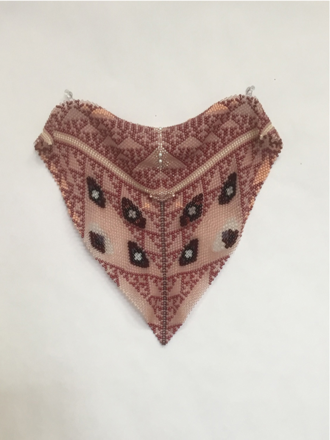
In my loomless hand-weaving practice, I use cellular automata rules in a repeated way, with simple heuristics guiding my work. As a result, I have internalized some fundamental insights about certain Cellular Automata. While these Rule heuristics seem obvious in retrospect, the formulations are quite different from what is seen in the literature, and they suggest a more fundamental perspective for appreciating how elementary CA Rules manifest. Over half of the 256 elementary Rules (at least 146 rules) have their origins in the fundamental, pre-symbolic dynamics I discuss here. For human makers, these heuristics are easily communicated in form and in action, and most are memorized easily. It is not difficult to imagine that some biologic systems can harness these heuristics with specific mechanics. Thinking of the CA Rules this way might also suggest experimental pathways; for example, to mimic how they were discovered and harnessed by nature as growth rules. As a by-product of many of these Rules, symmetry is maintained. Symmetry is a valuable functional affordance (low-cost error checking) and further mitigates in favor of these heuristic-based Rules. These heuristics may establish mechanisms of action, for explaining how and why these Rules play a significant role in the universe we perceive and experience.
Heuristic-based Classifications of CA Rules
Heuristic-based Classifications of CA Rules
Loomless weaving mechanics
Loomless weaving mechanics
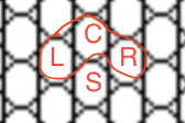
Many textile hand-making practices rely on a brick-like structure that is built in rows. One loomless bead-weaving technique is called “peyote stitch”, and it requires the maker to sew beads into the textile, one by one, placing each new bead in a nook that is formed by three beads.
This is an annotated illustration of a section of peyote stitch, with the left, center, and right bead indicated, as well as the new bead added below this triple (S):
In[]:=
Out[]=
In practice, beads are applied individually, row by row, either back and forth in a flat form, in nested rings, or in a spiral. The thread path is created by a needle passing through the L bead, stringing on a new S bead, and then passing through the R bead. The R bead then becomes the new L bead in the subsequent nook. This structure means that the L and R beads are adjacent to the new S bead, and the C bead is simply a passive place-holder and reference.
In flat weaving, the next row is woven in the opposite order, with the needle passing through the R bead, stringing on a new S bead, and then passing through the L bead.
In flat weaving, the next row is woven in the opposite order, with the needle passing through the R bead, stringing on a new S bead, and then passing through the L bead.
A simple difference-based heuristic
A simple difference-based heuristic
My own recent work involves the repeated use of a simple heuristic:
Given two possible bead colors (such as, light and dark), when determining the color of bead to apply (S):
- if the two adjacent beads (L and R) are the same, add a light bead
- if the two adjacent beads are different, add a dark bead
- if the two adjacent beads (L and R) are the same, add a light bead
- if the two adjacent beads are different, add a dark bead
In more technical terminology:
- if L = R, S = light
- if L<>R, S = dark
In this formulation, the light beads can be seen as the “default” bead color, forming the background for the pattern. The dark beads can be seen as the variant color, propagating to form the pattern.
- if L = R, S = light
- if L<>R, S = dark
In this formulation, the light beads can be seen as the “default” bead color, forming the background for the pattern. The dark beads can be seen as the variant color, propagating to form the pattern.
Rules 90, 60 and 102 are XOR and only require difference-detection
Rules 90, 60 and 102 are XOR and only require difference-detection
The heuristic described above is equivalent to the logic table for XOR, and it is also equivalent to Rule 90, where the center cell of the triple is silent. Rule 90 requires a system to detect a single local difference, and to adapt its response based on simple difference or similarity.
Here is the RulePlot for Rule 90:
In[]:=
RulePlot[CellularAutomaton[90]]
Out[]=
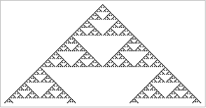
Here are the first 100 rows of the simple Rule 90 CA plot:
In[]:=
CellularAutomaton[90,{{1},0},100]//ArrayPlot
Out[]=
Two other Rules behave in a similar way. Rule 60 leaves the R bead silent, and assigns the color of the new bead S based on the difference between the L and C beads. Rule 102 references the R and C beads.
I want to mention here that the set of three XOR rules (60, 90, 102) produce a surprisingly stable result, in situations where mistakes are made. If the “silent” cell is chosen at random with equal probability, the resulting pattern resembles Rule 90. In the Appendix to this essay, I provide the code to experiment with how these (and any other Rules) might combine with each other. (See “ArrayPlots with varying Rules”)
I want to mention here that the set of three XOR rules (60, 90, 102) produce a surprisingly stable result, in situations where mistakes are made. If the “silent” cell is chosen at random with equal probability, the resulting pattern resembles Rule 90. In the Appendix to this essay, I provide the code to experiment with how these (and any other Rules) might combine with each other. (See “ArrayPlots with varying Rules”)
Here is the RulePlot for Rule 60:
In[]:=
RulePlot[CellularAutomaton[60]]
Out[]=
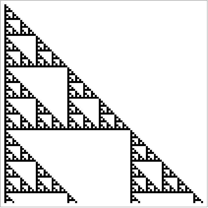
Here are the first 100 rows of the simple Rule 60 CA plot:
In[]:=
CellularAutomaton[60,{{1},0},100]//ArrayPlot
Out[]=
Here is the RulePlot for Rule 102:
In[]:=
RulePlot[CellularAutomaton[102]]
Out[]=
Here are the first 100 rows of the simple Rule 102 CA plot:
In[]:=
CellularAutomaton[102,{{1},0},100]//ArrayPlot
Out[]=
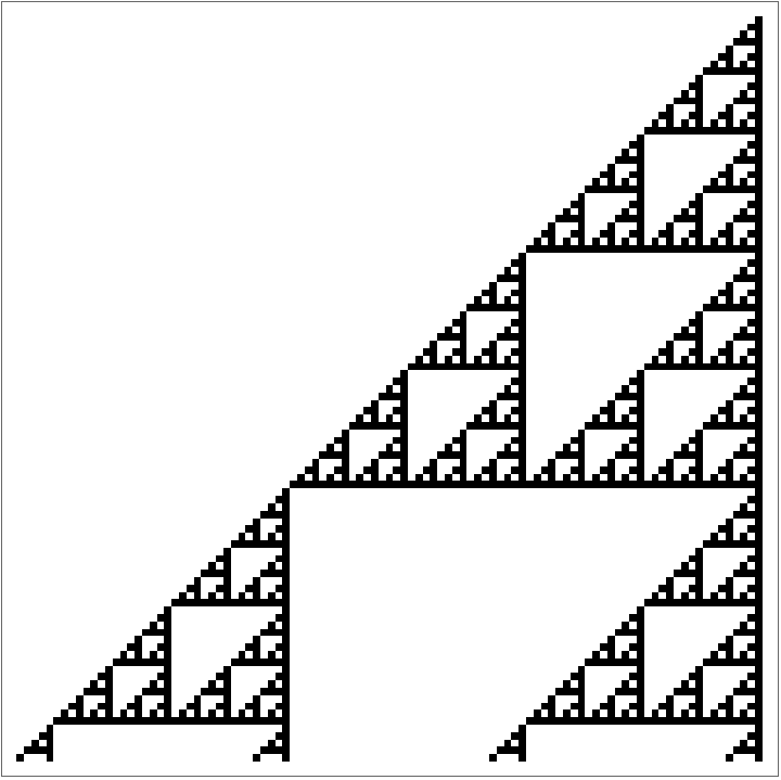
In this case, the “inverse” or complement of each Rule behaves in exactly the same way. The colors just switch roles in the story.
In the phrasing I use for weaving, the inverse of Rule 90 is expressed as:
In the phrasing I use for weaving, the inverse of Rule 90 is expressed as:
Given two possible bead colors (such as, light and dark), when determining the color of bead to apply (S):
- if the two adjacent beads (L and R) are the same, add a dark bead
- if the two adjacent beads are different, add a light bead
- if the two adjacent beads (L and R) are the same, add a dark bead
- if the two adjacent beads are different, add a light bead
Here is the RulePlot for 255-90 = Rule 165:
In[]:=
RulePlot[CellularAutomaton[165]]
Out[]=
Here are the first 100 rows of the simple Rule 165 CA plot:
Rule 30 as an OR/NOR switch
Rule 30 as an OR/NOR switch
Similar heuristics can be used to animate the weaving of other CA Rules. For example, Rule 30 can be woven as:
Given two possible bead colors (such as, light and dark), when determining the color of bead to apply (S):
- always use the opposite of the left bead color, unless C and R are both light beads.
- always use the opposite of the left bead color, unless C and R are both light beads.
Here is the RulePlot of Rule 30:
Here is the first 100 rows of the simple Rule 30 CA plot:
This suggests that the following Rules are related to Rule 30:
* Rule 17 can be understood as NOT OR on the Center and Right cells, independent of the value in the Left cell.
* Rule 238 can be understood as OR on the Center and Right cells, independent of the value of the Left cell.
Here, Rule 17 and Rule 238 are kind of inverses of each other, but their behavior is very different.
Here is the RulePlot of Rule 17:
Here is the RulePlot of Rule 238:
Here are ArrayPlots for both Rule 17 and Rule 238
The idea that Rule 30 is a kind of combination of the above two predictable Rules is quite stunning.
Interpreting Rule 30 as a switch between NOT OR and OR also points us to Rule 225, which interprets the Left cell “switch” in the other way.
Interpreting Rule 30 as a switch between NOT OR and OR also points us to Rule 225, which interprets the Left cell “switch” in the other way.
Given two possible bead colors (such as, light and dark), when determining the color of bead to apply (S):
- always use the same as the left bead color, unless C and R are both light beads.
- always use the same as the left bead color, unless C and R are both light beads.
Here is the RulePlot of Rule 225:
Here is the first 300 rows of the simple Rule 225 CA plot:
To see Rule 225 related to Rule 30 in this way is a shock. It appears as a distorted Sierpinski arrangement, seen from an oblique angle. One is reminded of the Holbein painting, The Ambassadors, with a skull that can only be seen properly if the viewer positions themselves at an awkward angle.
Given two possible bead colors (such as, light and dark), when determining the color of bead to apply (S):
- always use the opposite of the right bead color, unless L and C are both light beads.
- always use the opposite of the right bead color, unless L and C are both light beads.
Here is the RulePlot of Rule 86:
Here is the first 100 rows of the simple Rule 86 CA plot:
Here is the first 100 rows of the simple Rule 54 CA plot:
Here is the first 100 rows of the simple Rule 54 CA plot:
Here is a plot of random initial conditions for Rule 54, to “shake the tree”:
Rule 110 operates as an XOR/OR Switch
Rule 110 operates as an XOR/OR Switch
In a similar way, Rule 110 can be seen as a simple combination of XOR and OR logic. Rule 110 can be memorized easily, and requires no symbolic language to communicate; it relies on a default growth behavior, the assessment of difference, and the ability to interpret a switch that indicates the growth behavior response to difference or similarity. In essence, Rule 110 is a Rule that uses the Left cell to choose the logic rule to apply to the other two cells.
Here is the RulePlot of Rule 110:
As a weaving heuristic, Rule 110 can be expressed as follows:
- If the left bead is the “default” color (light), then the new bead is the “variant” color (dark) if the variant already appears in any of the other two beads (center or right).
- If the left cell is a “variant” color (dark), then output the variant type if the other two cells are different.
- Otherwise, output the default color (light).
- If the left cell is a “variant” color (dark), then output the variant type if the other two cells are different.
- Otherwise, output the default color (light).
Here are the first 100 rows of the simple Rule 110 CA plot:
This formulation suggests that Rules 102 and 238 have a relationship with Rule 110:
* Rule 102 can be understood as XOR on the Center and Right cells, independent of the value in the Left cell.
* Rule 238 can be understood as OR on the Center and Right cells, independent of the value of the Left cell.
* Rule 102 can be understood as XOR on the Center and Right cells, independent of the value in the Left cell.
* Rule 238 can be understood as OR on the Center and Right cells, independent of the value of the Left cell.
Here is the RulePlot of Rule 102:
Here is the RulePlot of Rule 238:
Here is the ArrayPlot of both 102 and 238:
Here is the RulePlot of Rule 230:
Unlike Rule 110, the result of the Rule 230 version of XOR/OR combination is completely predictable (at least with simple initial conditions), which is another surprising result.
Here is the ArrayPlot of Rule 230:
Here is the ArrayPlot of Rule 230 with random initial conditions:
I note that there are other ways automata can act as an XOR/OR switch, using their Center or Right cells as the switch indicator. Rules 124, 188, 122, and 218 can be seen as exhibiting XOR/OR switch mechanics, using their Right or Center cell value as the switch.
Rule 124 is very similar to Rule 110, with the “switch” based on the Right cell. However, Rule 122 is very predictable, with the switch in the Center cell.
Rule 188 is similar to Rule 230 (boring, predictable), but Rule 218 shows classic Sierpinski-like predictability under a simple starting condition.
Also notable is that, under more complex starting conditions, Rules 122 and 218 lose their delicate balance. Rule 122 becomes more complex, and Rule 218 succumbs to large areas with little change.
Here is the RulePlot of Rule 124:
Here is the ArrayPlot of Rule 124
Here is the RulePlot of Rule 122:
Here is the ArrayPlot of Rule 122
Here is the RulePlot of Rule 188:
Here is the ArrayPlot of Rule 188
Here is the RulePlot of Rule 218:
Here is the ArrayPlot of Rule 218
I wanted to “shake the tree” to see how some of these simple rules behave with more complex initial conditions.
Here is the ArrayPlot of Rule 218 with random initial conditions:
Here is the ArrayPlot of Rule 122 with random initial conditions:
The special case of Rule 105 and 150
The special case of Rule 105 and 150
Rule 105 follows an unusually flexible “switch” pattern:
Using the Left cell of the triple as a “switch”,
If C <> R (center and right cells are different), use the left cell’s value (L) as the output color (or value).
If C=R (center and right cells are the same), use the “opposite” color or value (1-L).
In other words, this suggests that Rule 105 is similar to XOR on the Center and Right cells, with the output set by the value of the Left cell.
In fact, the same heuristic can be applied, no matter which cell is chosen as the “switch”.
Here is the RulePlot of Rule 105:
Here are the first 100 rows of the simple Rule 105 CA plot:
Rule 150, the “inverse” of Rule 150, can be described in a similar way:
If C=R (center and right cells are the same), use the left cell’s value (L) as the output color.
If C <> R (center and right cells are different), use the “opposite” color (1-L).
Either L or R can be used as the “switch” for Rule 150, but if the Center cell is used as the switch, we get Rule 154.
This is surprising. The “inverse” of Rule 105 has such a different behavior. It is not simply the “inverse” of Rule 105.
Here is the RulePlot of Rule 150:
Here is the first 100 rows of the simple Rule 150 CA plot:
Here is the RulePlot of Rule 154:
Here are the first 100 rows of the simple Rule 154 CA plot:
In addition, the inverse of Rule 154 is Rule 101. Rule 101 can be described as using the Center cell as a switch. It outputs the switch color (C) when the other two cells differ, and it outputs the opposite (1-C) when they match. This works only with the Center cell as the switch.
Here is the RulePlot of Rule 101:
Here are the first 100 rows of the simple Rule 101 CA plot:
A manipulate to develop other Rules
A manipulate to develop other Rules
In the appendix is a manipulate that shows how any set of basic logic rules can be combined to create a set of Cellular Automata.
The key idea is that one element of each binary tuple is a switch. The value of the switch determines the logic rule that is applied to the remaining elements of the tuple.
My code calculates the combinations of Rules that result from selected Rules, across all three potential switch positions. One can account for 88 of the 256 rules using this approach.
An even more general approach to generating CA rules
An even more general approach to generating CA rules
The observations above suggest an even more general approach to generating CA rules. In any triple, the switch could vary. The switch is used to determine what is effectively the “truth” value that is output from the application of a simple logic rule, applied to the remaining two elements of the triple.
Similarly, in any triple, the silent cell could vary. A simple logic rule would then apply to the remaining two elements of the triple.
For example, an xOrs Cluster emerges from the following mechanism, wherein:
Neighborhood: Each Cellular Automata rule considers a tuple (L, C, R), where L (left), C (center), and R (right) are binary values (0 or 1).
Silent Cell: For each tuple, one of the three cells is designated as silent, chosen independently (effectively at random during rule definition).
Output Rule: The output (next state, S) is the XOR of the two non-silent cells. For example:
If R is silent, S = XOR(L, C).
If C is silent, S = XOR(L, R).
If L is silent, S = XOR(C, R).
Implicit Constraints: For the tuple 111, all XOR pairs yield 0, so the output is always 0. Similarly, for tuple 000, the output is 0. For the other six tuples (110, 101, 100, 011, 010, 001), the output can be 0 or 1, depending on which cell is silent.
In the appendix, I show the code that produces the 64 distinct CAs that result from applying XOR across all permutations of silent cells across the 8 possible elementary triples. Only 6 of the 64 xOr cluster rules are contained in the 88 Rules that can be made from the elementary logic builder.
The same approach with AND and OR reveals 8 Rules, 4 of which are not in the 88 Rules that can be made from the elementary logic builder, but all 8 are included in the 64 distinct CAs that are in the xOrs Cluster.
Relationship to other formulations
Relationship to other formulations
I can account for at least 88 + 64 - 6 = 146 cellular automata rules using these techniques. While similar to other formulations, I believe this may be a novel way to describe many of the elementary Cellular Automata.
In a note in NKS (page 951), Stephen Wolfram provides a logic statement as an alternative formulation of Rule 225. Page 869 of NKS (Notes for Chapter 2) also suggests logic expressions and algebraic definitions for Rule 110 (and some others). However, I believe the formulation I propose is a bit different. The idea of a switch and the mechanics of these formulations suggest paths to developing deeper intuition, when it comes to many Rules.
In a note in NKS (page 951), Stephen Wolfram provides a logic statement as an alternative formulation of Rule 225. Page 869 of NKS (Notes for Chapter 2) also suggests logic expressions and algebraic definitions for Rule 110 (and some others). However, I believe the formulation I propose is a bit different. The idea of a switch and the mechanics of these formulations suggest paths to developing deeper intuition, when it comes to many Rules.
On page 869, there are notes that address algebraic expressions and logic statements that are similar (but not identical) to those outlined here.
Appendix
Appendix
ArrayPlots with varying Rules
ArrayPlots with varying Rules
A manipulate to develop other Rules
A manipulate to develop other Rules
This manipulate shows how any set of basic logic rules can be combined to create a set of Cellular Automata.
The key idea is that one element of each binary tuple is a switch. The value of the switch determines the logic rule that is applied to the remaining elements of the tuple.
My code calculates the combinations of Rules that result from selected logic gates, across all three potential switch positions.
Defining the xORs cluster
Defining the xORs cluster
The xOrs Cluster emerges from the following mechanism:
Neighborhood: Each Cellular Automata rule considers a tuple (L, C, R), where L (left), C (center), and R (right) are binary values (0 or 1).
Silent Cell: For each tuple, one of the three cells is designated as silent, chosen independently (effectively at random during rule definition).
Output Rule: The output (next state, S) is the XOR of the two non-silent cells. For example:
If R is silent, S = XOR(L, C).
If C is silent, S = XOR(L, R).
If L is silent, S = XOR(C, R).
Generate the canonical list of binary tuples:
Define a function to process a single triple with a silent cell:
Apply the function to all triples with a specified silent position for each tuple:
Generate all rules in the xOrs Clusters:
Execute to generate and display the xOrs Cluster:
Defining the ANDs cluster
Defining the ANDs cluster
The ANDs Cluster emerges from the following mechanism:
Neighborhood: Each Cellular Automata rule considers a tuple (L, C, R), where L (left), C (center), and R (right) are binary values (0 or 1).
Silent Cell: For each tuple, one of the three cells is designated as silent, chosen independently (effectively at random during rule definition).
Output Rule: The output (next state, S) is the XOR of the two non-silent cells. For example:
If R is silent, S = AND(L, C).
If C is silent, S = AND(L, R).
If L is silent, S = AND(C, R).
Generate the canonical list of binary tuples:
Define a function to process a single triple with a silent cell:
Apply the function to all triples with a specified silent position for each tuple:
Generate all rules in the ANDs Clusters:
Execute to generate and display the ANDs Cluster:
Defining the ORs cluster
Defining the ORs cluster
The Ors Cluster emerges from the following mechanism:
Neighborhood: Each Cellular Automata rule considers a tuple (L, C, R), where L (left), C (center), and R (right) are binary values (0 or 1).
Silent Cell: For each tuple, one of the three cells is designated as silent, chosen independently (effectively at random during rule definition).
Output Rule: The output (next state, S) is the OR of the two non-silent cells. For example:
If R is silent, S = OR(L, C).
If C is silent, S = OR(L, R).
If L is silent, S = OR(C, R).
Generate the canonical list of binary tuples:
Define a function to process a single triple with a silent cell:
Apply the function to all triples with a specified silent position for each tuple:
Generate all rules in the Ors Clusters:
Execute to generate and display the Ors Cluster:
Cite This Notebook
Cite This Notebook
Heuristic-based classifications of cellular automata rules
by Ellynne DEC
Wolfram Community, 20 June 2025
https://community.wolfram.com/groups/-/m/t/3482887
by Ellynne DEC
Wolfram Community, 20 June 2025
https://community.wolfram.com/groups/-/m/t/3482887