In the first blog, we walked you through how to model an electric vehicle (EV) driveline and battery to understand battery dynamics using the open-source EHPTlib library, focusing on streamlining your workflow and obtaining meaningful results.
In this blog, we’ll continue our journey by building upon the previous battery thermal dynamics outcomes. In real-life battery thermal management system applications, sensors are placed on the battery to measure spatial heat propagation. This practice naturally raises the question of how certain and dependable these measurements are.
In this second part of the EV series, we’ll outline a practical workflow for obtaining reliable measurements that take into account the spatial dynamics of the battery
Importing the System Model
Importing the System Model
As a first step we again import open source system model library . When we do this, then there is no need to open the System Modeler application separately. The model library provides us with several premade models.
"EHPTlib.mo"
Import the Library:
In[]:=
modelFileName=FileNameJoin[{NotebookDirectory[],"package.mo"}];model=Import[modelFileName]
Out[]=
Exploring the EV Model
Exploring the EV Model
We choose the “BatteryModern” model from the library’s examples with an updated battery. Here’s how to visualize its diagram and inspect its properties:
In[]:=
model=SystemModel["EHPTlib.Examples.EV.BatteryModern"];model["Diagram"]
Out[]=
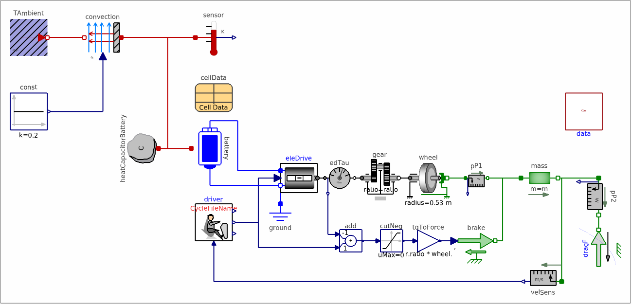
Here we see the comprehensive representation of the Tesla Model S structure, including its battery, drive system, and transmission components. Note that we have added also convection term. This allows us to model the car’s dynamics accurately and fine-tune its performance in different scenarios.
For further insight, you are encouraged to read the library documentation.
For further insight, you are encouraged to read the library documentation.
Visualizing Some Simulation Results
Visualizing Some Simulation Results
The result is a that contains all simulation results of interest.
We can visualize any variable in the stored data but let’s start with default System Modeler plots with the function:
In[]:=
sim=SystemModelSimulate[model]
Out[]=
SystemModelSimulationData


In[]:=
SystemModelPlot[sim,"Vehicle speed",ImageSize->Medium,PlotRange->Full]
Out[]=
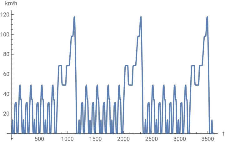

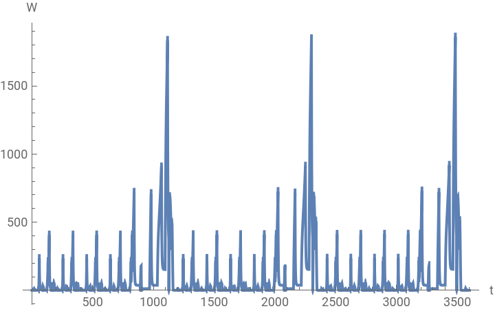
Here, we observe the battery temperature and car velocity. We have again used the benchmark velocity profile, New European Driving Cycle (NEDC).
Revisit Transient PDE Battery Simulation with FEM
Revisit Transient PDE Battery Simulation with FEM
In the previous post, we delved deeper into modeling an electric vehicle (EV) using a heat transfer Partial Differential Equation (PDE) model for simulation. The PDE was solved with the finite element method (FEM) to visualize the temperature distribution across the battery body and understand its spatial dynamics. This simulation provided insights into the transient behavior related to heat propagation.
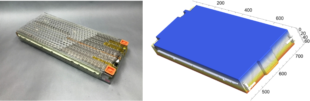
Below, we observe the transient behavior response over the spatial geometry of the battery. As expected, the temperature varies over the body and is not uniform.
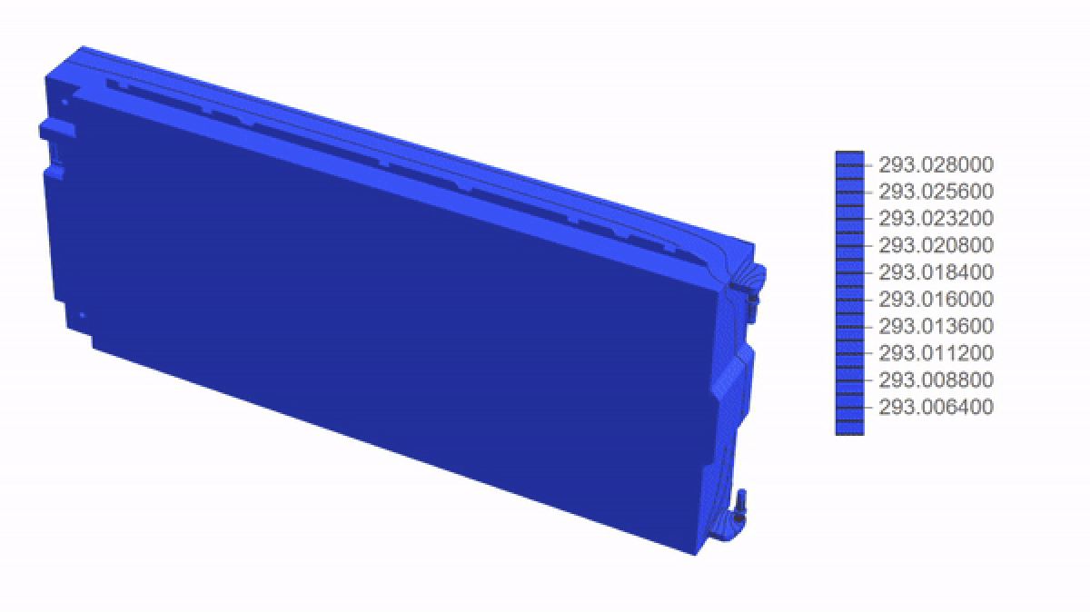
Let’s import the transient analysis results from the previous post:
In[]:=
Tfun=InterpolatingFunction
;

At this point, we calculate the mean and standard deviation to introduce these statistical characteristics into our lumped model.
In[]:=
Mean[Mean[Tfun["ValuesOnGrid"]]]Mean[StandardDeviation[Tfun["ValuesOnGrid"]]]
Out[]=
288.227
Out[]=
0.52719
One might ask, “What is the end game here?”
The goal is to incorporate these PDE characteristics into a lumped model. Since capturing spatial dynamics with temperature sensors across the battery is crucial, multiple sensors are placed at different locations to gather various point temperature measurements and possibly create interpolating relations between these positions. For instance, the Tesla Model S uses 32 temperature sensors on its battery.
Our idea is to use a single sensor with these incorporated variations in a system-level model.
Incorporating PDE dynamics into Lumped model
Incorporating PDE dynamics into Lumped model
In this section, we’ll show how to add these PDE dynamics to an electric vehicle’s battery model. To test the idea proposed above, we add a deviation component to the BatteryModern model and sum it with the temperature sensor output. This new model can be found in the library under EHPTlib.Examples.EV.EVwtUncertainties. You can open it as follows:
In[]:=
model=SystemModel["EHPTlib.Examples.EV.EVwtUncertainties"];model["Diagram"]
Out[]=
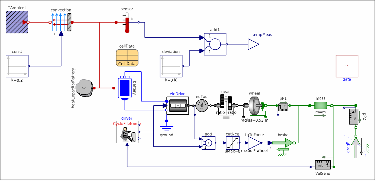
Now it is time to add PDE characteristics as deviations to our measurement readings. This can be done using the SystemModelUncertaintyPlot function.
Here, we’ll assume this distribution follows a normal Gaussian distribution. However, further analysis can determine whether the PDE temperature data exhibits binomial characteristics or another type of distribution.
Here, we’ll assume this distribution follows a normal Gaussian distribution. However, further analysis can determine whether the PDE temperature data exhibits binomial characteristics or another type of distribution.
In[]:=
SystemModelUncertaintyPlot[model,<|"Outputs"->{"tempMeas"},"ParameterValues"->{"deviation.k"->QuantityDistribution[TruncatedDistribution[{0,Infinity},NormalDistribution[0,Mean[StandardDeviation[Tfun["ValuesOnGrid"]]]]],"Kelvins"]},"InterpolationPoints"->200|>]
The plot shows the temperature measurements (tempMeas) over time, incorporating uncertainties derived from the PDE simulation. The mean temperature gradually increases while the uncertainty bands widen, indicating growing variability in temperature measurements, which underscores the need for effective thermal management in EV batteries.
This setup allows us to analyze the transient heat transfer and incorporate spatial variations into our lumped model, enhancing the reliability of the battery thermal management system.
Conclusion
Conclusion
In this post, we advanced our understanding of battery thermal dynamics in electric vehicles by integrating PDE-based simulations with system-level models. By incorporating statistical variations into our lumped model, we demonstrated a practical workflow for obtaining reliable temperature measurements that account for the PDE dynamics of the battery. This approach highlights the critical importance of effective thermal management in ensuring the performance and safety of EV batteries.
CITE THIS NOTEBOOK
CITE THIS NOTEBOOK
Electrical vehicle insights: battery management system —measurement uncertainties
by Vedat Senol, Sergio Vargas and Oliver Ruebenkönig
Wolfram Community, STAFF PICKS, July 25, 2024
https://community.wolfram.com/groups/-/m/t/3234411
by Vedat Senol, Sergio Vargas and Oliver Ruebenkönig
Wolfram Community, STAFF PICKS, July 25, 2024
https://community.wolfram.com/groups/-/m/t/3234411