ABSTRACT (original article): Conic sections are commonly used in reflective X-ray optics. Hyperbolic mirrors can focus a converging light source and are frequently paired with elliptical or parabolic mirrors in Wolter type configurations. This paper derives the closed-form expression for a mirror-centered hyperbolic shape, with zero-slope at the origin. Combined with the slope and curvature, such an expression facilitates metrology, manufacturing and mirror-bending calculations. Previous works consider ellipses, parabolas, magnifying hyperbolas or employ lengthy approximations. Here, the exact shape function is given in terms of the mirror incidence angle and the source and image distances. CITATION (original article): Torras, J.-P. (2024). Mirror-centered representation of a focusing hyperbolic mirror for X-ray beamlines. J. Synchrotron Rad. 31, 1464-1468. https://doi.org/10.1107/S1600577524009603
This workbook lays out the derivation of a “Mirror-centered representation of focusing hyperbolic mirror for X-ray beamlines.” When referring to “Equation XX" in this workbook, we mean the numbered equation in Torras (2024). We suggest reading the paper along with this workbook for best comprehension. The goal of this workbook is to show the use of various geometric laws to generate a quadratic equation of the form Ay^2+By+c=0, (note the use of lowercase c to avoid variable conflicts), and then solve for a function y(x) with inputs o, p, and q using the quadratic formula (we use o to represent theta throughout this workbook). We seek to present the final equation in a simple, compact form. Achieving this form requires several intermediate steps.
We start with Equation 6. Equation 6 is very difficult to work with and must be parsed out. Following the logic in the Torras (2024), we substitute in terms m and n.
We start with Equation 6. Equation 6 is very difficult to work with and must be parsed out. Following the logic in the Torras (2024), we substitute in terms m and n.
In[]:=
Clear[a,k,x,G,H,dHdx,d2Hdx2,y,dy,dy2,p,q,m,n,L,o];
At this point, we have Equation 8, 2a=m^(1/2)-n^(1/2). We separate the square roots, 2a+n^(1/2)=m^(1/2), and square both sides:
In[]:=
Expand[(2a+n^(1/2))^2]Expand[(m^(1/2))^2]
Out[]=
4+4a
2
a
n
+nOut[]=
m
Next isolate the remaining n^(1/2) on side of the equation, 4 a =m-4 -n, and square both sides again:
n
2
a
In[]:=
Expand[4a-n)^2]
n
^2]Expand[(m-42
a
Out[]=
16n
2
a
Out[]=
16-8m++8n-2mn+
4
a
2
a
2
m
2
a
2
n
Gather terms on one side of the equation to equal zero, and simplify as in Equation 9:
In[]:=
Simplify[16-8m++8n-2mn+-16n]
4
a
2
a
2
m
2
a
2
n
2
a
Out[]=
16+-8(m+n)
4
a
2
(m-n)
2
a
Next we substitute back the y, x, p, q, and o terms from Equations 5, 7a, and 7b. We expand and collect about y:
In[]:=
a=(q-p)/2;m=(y-q*Sin[o])^2+(x-q*Cos[o])^2;n=(y-(-p)*Sin[o])^2+(x-p*Cos[o])^2;Collect[Expand[16+-8(m+n)],y]
4
a
2
(m-n)
2
a
Out[]=
4
p
3
p
2
p
2
q
3
q
4
q
2
p
2
x
2
x
2
q
2
x
3
p
2
p
2
q
3
q
4
p
2
Cos[o]
3
p
2
Cos[o]
2
p
2
q
2
Cos[o]
3
q
2
Cos[o]
4
q
2
Cos[o]
2
p
2
x
2
Cos[o]
2
x
2
Cos[o]
2
q
2
x
2
Cos[o]
3
p
3
Cos[o]
2
p
3
Cos[o]
2
q
3
Cos[o]
3
q
3
Cos[o]
4
p
4
Cos[o]
2
p
2
q
4
Cos[o]
4
q
4
Cos[o]
4
p
2
Sin[o]
3
p
2
Sin[o]
2
p
2
q
2
Sin[o]
3
q
2
Sin[o]
4
q
2
Sin[o]
3
p
2
Sin[o]
2
p
2
Sin[o]
2
q
2
Sin[o]
3
q
2
Sin[o]
4
p
2
Cos[o]
2
Sin[o]
2
p
2
q
2
Cos[o]
2
Sin[o]
4
q
2
Cos[o]
2
Sin[o]
4
p
4
Sin[o]
2
p
2
q
4
Sin[o]
4
q
4
Sin[o]
2
y
2
p
2
q
2
p
2
Sin[o]
2
Sin[o]
2
q
2
Sin[o]
3
p
2
p
2
q
3
q
2
p
2
q
3
p
2
Cos[o]
2
p
2
Cos[o]
2
q
2
Cos[o]
3
q
2
Cos[o]
3
p
3
Sin[o]
2
p
3
Sin[o]
2
q
3
Sin[o]
3
q
3
Sin[o]
We now have an Equation of the form Ay^2+By+c=0. Next is the "compacting process." The most compact form of the above requires some trial and error to determine which terms to collect about. From the output above, we manually gather terms as follows in Equation 11:
In[]:=
A=Simplify[Collect[-4+8pq-4+4+8pq+4,Sin[o]]]B=Simplify[Collect[-4Sin[o]+12qSin[o]-12pSin[o]+4Sin[o]-8xCos[o]Sin[o]+8xCos[o]Sin[o]+4Sin[o]+4qSin[o]-4pSin[o]-4Sin[o]+4+4q-4p-4,Sin[o]]]c=Simplify[Collect[-4q+6-4p+-4+8pq-4+4xCos[o]-4qxCos[o]-4pxCos[o]+4xCos[o]-2+4q-4+4p-2+4-8pq+4-4x+4qx+4px-4x+-2+-2+4q-4+4p-2-4xCos[o]+4qxCos[o]+4pxCos[o]-4xCos[o]+2-4+2+-2+,x]]
2
p
2
q
2
p
2
Sin[o]
2
Sin[o]
2
q
2
Sin[o]
3
p
2
p
2
q
3
q
2
p
2
q
3
p
2
Cos[o]
2
p
2
Cos[o]
2
q
2
Cos[o]
3
q
2
Cos[o]
3
p
3
Sin[o]
2
p
3
Sin[o]
2
q
3
Sin[o]
3
q
3
Sin[o]
4
p
3
p
2
p
2
q
3
q
4
q
2
p
2
x
2
x
2
q
2
x
3
p
2
p
2
q
3
q
4
p
2
Cos[o]
3
p
2
Cos[o]
2
p
2
q
2
Cos[o]
3
q
2
Cos[o]
4
q
2
Cos[o]
2
p
2
x
2
Cos[o]
2
x
2
Cos[o]
2
q
2
x
2
Cos[o]
3
p
3
Cos[o]
2
p
3
Cos[o]
2
q
3
Cos[o]
3
q
3
Cos[o]
4
p
4
Cos[o]
2
p
2
q
4
Cos[o]
4
q
4
Cos[o]
4
p
2
Sin[o]
3
p
2
Sin[o]
2
p
2
q
2
Sin[o]
3
q
2
Sin[o]
4
q
2
Sin[o]
3
p
2
Sin[o]
2
p
2
Sin[o]
2
q
2
Sin[o]
3
q
2
Sin[o]
4
p
2
Cos[o]
2
Sin[o]
2
p
2
q
2
Cos[o]
2
Sin[o]
4
q
2
Cos[o]
2
Sin[o]
4
p
4
Sin[o]
2
p
2
q
4
Sin[o]
4
q
4
Sin[o]
Out[]=
-4+4
2
(p-q)
2
(p+q)
2
Sin[o]
Out[]=
-8(p-q)(-2pq+(p+q)xCos[o])Sin[o]
Out[]=
-4
2
(p-q)
2
x
2
Sin[o]
We now have more compact quadratic terms, and can apply the quadratic formula to find the mirror surface height as in Equation 12:
In[]:=
y[x_]=Simplify[(-B-(B^2-4*A*c)^(1/2))/(2*A)]
Out[]=
(p-q)(-2pq+(p+q)xCos[o])Sin[o]-2
pq(pq+-(p+q)xCos[o])
2
(p-q)
2
x
2
Sin[o]
-+
2
(p-q)
2
(p+q)
2
Sin[o]
Note that we arbitrarily choose the negative root case for this explanation. Next, it is trivial to substitute in a=q-p and 2k=q+p to generate an even more compact equation as shown in Equation 13. Furthermore, this form removes the need to switch between root cases.
In[]:=
a=q-p;k=(q+p)/2;y[x_]=a*Sin[o]/(k^2*Sin[o]^2-a^2)*(p*q-k*x*Cos[o]-Sqrt[p*q]*Sqrt[p*q+x^2-2*k*x*Cos[o]])
Out[]=
(-p+q)pq-(p+q)xCos[o]-
1
2
pq
pq+-(p+q)xCos[o]
Sin[o]2
x
-+
2
(-p+q)
1
4
2
(p+q)
2
Sin[o]
The derivatives, mirror slope and curvature, are found next:
In[]:=
dy[x_]=D[y[x],x]dy2[x_]=D[y[x],{x,2}]
Out[]=
(-p+q)-(p+q)Cos[o]-Sin[o]
1
2
pq
(2x-(p+q)Cos[o])2
pq+-(p+q)xCos[o]
2
x
-+
2
(-p+q)
1
4
2
(p+q)
2
Sin[o]
Out[]=
-+Sin[o]
pq
(-p+q)-2
(2x-(p+q)Cos[o])
4
3/2
pq+-(p+q)xCos[o]
2
x
1
pq+-(p+q)xCos[o]
2
x
-+
2
(-p+q)
1
4
2
(p+q)
2
Sin[o]
By recognizing that certain collections of terms (Equations 14a-14d) reoccur in these Equations, with some pen and paper effort, we can again simplify and compact these large equations into significantly more manageable chunks as defined in Equations 15-17.
In[]:=
G=a*Sin[o]/(k^2*Sin[o]^2-a^2);H=(p*q+x^2-2*k*x*Cos[o])^(1/2);dHdx=(x-k*Cos[o])/H;d2Hdx2=(1-dHdx^2)/H;
Equations 15-17, note their equivalence to the previous height, slope, and curvature equations:
In[]:=
yCheck=G*(p*q-k*x*Cos[o]-(p*q)^(1/2)*H)dyCheck=G*(-k*Cos[o]-(p*q)^(1/2)*dHdx)dy2Check=-G*(p*q)^(1/2)*d2Hdx2
Out[]=
(-p+q)pq-(p+q)xCos[o]-
1
2
pq
pq+-(p+q)xCos[o]
Sin[o]2
x
-+
2
(-p+q)
1
4
2
(p+q)
2
Sin[o]
Out[]=
(-p+q)(-p-q)Cos[o]-(p+q)Cos[o]Sin[o]
1
2
pq
x-1
2
pq+-(p+q)xCos[o]
2
x
-+
2
(-p+q)
1
4
2
(p+q)
2
Sin[o]
Out[]=
-Sin[o]+
pq
(-p+q)1-2
x-(p+q)Cos[o]
1
2
pq+-(p+q)xCos[o]
2
x
pq+-(p+q)xCos[o]
-2
x
2
(-p+q)
1
4
2
(p+q)
2
Sin[o]
As proof, these equations are checked for equivalence:
In[]:=
FullSimplify[y[x]==yCheck]FullSimplify[dy[x]==dyCheck]FullSimplify[dy2[x]==dy2Check]
Out[]=
True
Out[]=
True
Out[]=
True
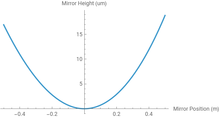
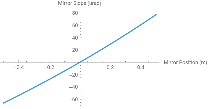
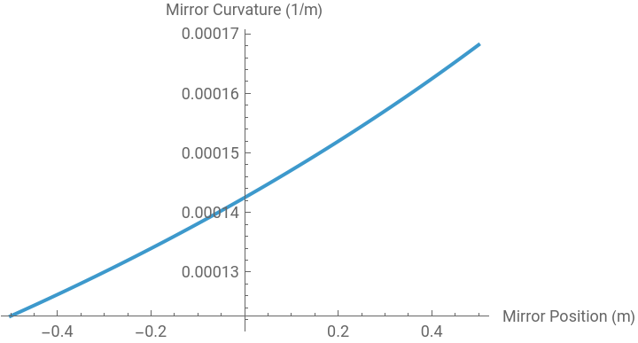
Below, we present an example using these equations. L is the mirror length, typically less than 2 meters, the source p and focus q distances are in meters, and the grazing angle o is in radians (o be should be well below 0.5 radians to ensure total external reflection of X-rays, errors may occur if much larger values are used). Note the zero height (y=0) and slope (dy=0) at the mirror center (x=0) as a sanity check. We can compare these plots to descriptions in Table 1 of Torras (2024) to see how the concavity (dy2) flips depending on whether p>q or q<p. The radius of curvature (a common figure of merit) is also provided.
The plots are scaled for visual clarity.
The plots are scaled for visual clarity.
In[]:=
L=0.5;p=100;q=5;o=0.003;Plot[10^6*y[x],{x,-L,L},AxesLabel{"Mirror Position (m)","Mirror Height (um)"}]Plot[10^6*dy[x],{x,-L,L},AxesLabel{"Mirror Position (m)","Mirror Slope (urad)"}]Plot[dy2[x],{x,-L,L},AxesLabel{"Mirror Position (m)","Mirror Curvature (1/m)"}]Plot[Abs[(1+dy[x])^(3/2)/dy2[x]],{x,-L,L},AxesLabel{"Mirror Position (m)","Radius of Curvature (m)"}]
Out[]=
Out[]=
Out[]=
Now p and q are flipped to highlight the concavity flip.
CITE THIS NOTEBOOK
CITE THIS NOTEBOOK
Mirror-centered representation of a focusing hyperbolic mirror for X-ray beamlines
by Jean-Pierre Torras
Wolfram Community, STAFF PICKS, January 14, 2026
https://community.wolfram.com/groups/-/m/t/3606624
by Jean-Pierre Torras
Wolfram Community, STAFF PICKS, January 14, 2026
https://community.wolfram.com/groups/-/m/t/3606624