ORIGINAL ARTICLE: Marcelo Amaral, Richard Clawson, Klee Irwin, Quasicrystalline Spin Foam with Matter: Definitions and Examples. arXiv:2306.01964 [gr-qc]. https://doi.org/10.48550/arXiv.2306.01964.
Abstract: This notebook serves as a companion to the paper “Quasicrystalline Spin Foam with Fermions: Definitions and Examples [1].” In this work, we define quasicrystalline spin networks as a subspace within the standard Hilbert space of loop quantum gravity, effectively constraining the states to those that align with quasicrystal geometry. We further introduce quasicrystalline spin foam amplitudes, a variation of the EPRL spin foam model, in which the internal spin labels are constrained to correspond with the boundary data of quasicrystalline spin networks. We showcase calculations for some 3D examples and subsequently explore the 600-cell construction, a fundamental component of the 4D Elser-Sloane quasicrystal originating from the E8 lattice. For the 600-cell, we show details in the construction of the boundary 3D states, which involves dual SO(4) rotations to bring tetrahedra in different 3D spaces of the 600-cell to the same 3D space. For detailed discussions, motivations, references, and further elaboration, please refer to the accompanying paper.
Introduction
Introduction
In the mentioned article, we introduce quasicrystalline spin networks as a novel subspace of the conventional Hilbert space of loop quantum gravity, motivated by the intriguing properties of quasicrystals. We explore how these networks provide a natural constraint on the states of quantum geometry, which are selected according to the geometric properties of quasicrystals. Building on this framework, we define quasicrystalline EPRL spin foam amplitudes, a modified version of the EPRL spin foam model, in which the internal spin labels are constrained to match the boundary data of the quasicrystalline spin networks, which are represented by coherent states.
We start by presenting the methodology for constructing quasicrystalline spin networks and spin foam amplitudes, followed by the implementation and analysis of specific 3D examples. We then extend our investigation to the more complex 600-cell, a building block of the 4D Elser-Sloane quasicrystal derived from the E8 lattice. This rich structure provides a unique platform for studying the properties of quasicrystalline spin networks and their amplitudes in higher dimensions.
Moreover, we delve into the coupling of matter to the EPRL spin foam model and the SU(3) charge, which can be understood in the context of the unification gauge group E8. This perspective sheds light on the possible implications of quasicrystalline spin networks and amplitudes for the understanding of fundamental interactions and the structure of spacetime.
In conclusion, our study paves the way for a deeper understanding of the interplay between quasicrystals, spin networks, and the EPRL spin foam model, offering new perspectives on the quantum geometry and the unification of fundamental forces.
Quasicrystalline Spin Network and Foam: Definitions
Quasicrystalline Spin Network and Foam: Definitions
Quasicrystalline Spin Network: Subset QSN(j) of LQG states where the spin quantum numbers j's and SU(2) states are compatible with 3D quasicrystal tiling geometry.
Quasicrystalline Spin Foam: Sum over tiling configurations compatible with the QSN(j) boundary states.
Quasicrystalline Spin Foam: Sum over tiling configurations compatible with the QSN(j) boundary states.
3D Quasicrystalline Spin Foam
3D Quasicrystalline Spin Foam
In[]:=
SetOptions[Graphics3D,Boxed->False,SphericalRegion->True];
3D Spin Foam
3D Spin Foam
For quantum gravity in three dimensions we consider three valent SU(2) spin network states and the 3D spin foam models boil down to the Ponzano-Regge model with SU(2) symmetry [2]:()(2+1) {6j} (1)which can be interpreted as the partition function or if we fix the boundary as transition amplitudes or observables of the theory [3]. The quantum numbers j from SU(2) representation theory are associated to the faces of the 2-complex dual of the triangulation . The dual is taken to be: Tetrahedron Vertices, Triangle Edge, Segment Face. The vertex amplitude is the Wigner {6j} symbol of angular momentum theory and is the sum of the spins of the faces adjacent to the vertex v. Let us reproduce the celebrated result that the vertex amplitude leads to the Regge's action in the limit of large spin. We remember that geometry is quantized in this loop quantum gravity framework. The area spectrum for example is given by
W
△
j
l
N
△
∑
j
f
∏
f
j
f
(-1)
j
f
∏
v
j
v
(-1)
j
v
In[]:=
lqgArea[j_,β_]:=βSqrt[j(j+1)]
In[]:=
c=UnitConvert[Quantity["SpeedOfLight"]]//N;hbar=UnitConvert[Quantity["ReducedPlanckConstant"]]//N;G=UnitConvert[Quantity["GravitationalConstant"]]//N;planckArea=hbar*G/c^38PihbarG/c^3;
Out[]=
with usually β=γ planckArea, where γ is the Barbero–Immirzi parameter, a free parameter of the theory, which can be fixed in different ways, for example from [4]
In[]:=
γ=Log[GoldenRatio]/Pi//N
Out[]=
0.153174
In[]:=
Log2[GoldenRatio]/Pi//N
Out[]=
0.220984
So the classical limit ♄ 0, imply j ∞ maintaining the physical area constant. Let us look the classical limit of the vertex amplitude considering all 6 spins equal to fixed j and then introduce a scaling parameter λ. The analytical result for , with a tetrahedron of length (j+1/2), dihedral angle of ArcCos[1/3], the Regge' action S=
{6j}
j⟶∞
3(j+1)ArcCos
1
3
Ava=Table(1/(Sqrt[12PiVolume[Tetrahedron[j+1/2]]]))Cos3(j+1)ArcCos+Pi4,{j,0,100};ReggesActionOsc=TableCos3(j+1)ArcCos+Pi4,{j,0,100};ListPlot[Ava,AxesLabel->{"Scale λ ","{6j} analytical limit"},PlotRange->All]ListPlot[ReggesActionOsc,AxesLabel->{"Scale λ ","{6j} analytical limit Regge"},PlotRange->All]
1
3
1
3
Out[]=
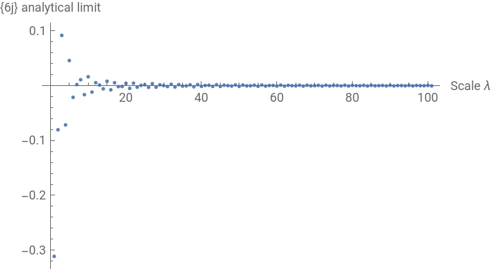
Out[]=
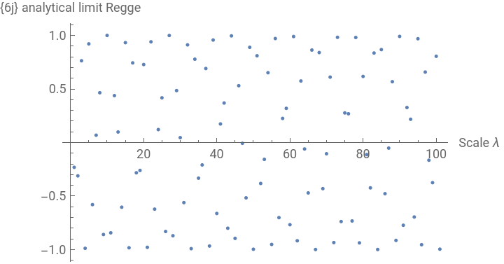
Now addressing directly the limit of the vertex amplitude numerically:
In[]:=
j=1;Av=Table[SixJSymbol[{λj,λj,λj},{λj,λj,λj}],{λ,0,100}];AvOsc=Table[(Sqrt[12PiVolume[Tetrahedron[λ+1/2]]])SixJSymbol[{λj,λj,λj},{λj,λj,λj}],{λ,0,100}];ListPlot[Av,AxesLabel->{"Scale λ ","{6j}"},PlotRange->All]ListPlot[AvOsc,AxesLabel->{"Scale λ ","{6j}"},PlotRange->All]
Out[]=
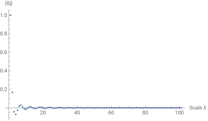
Out[]=
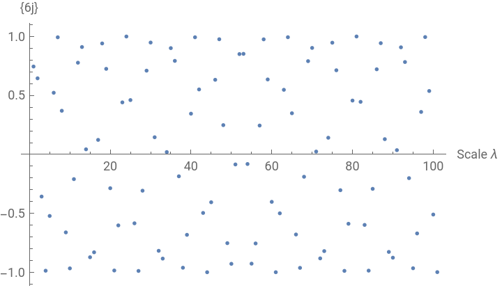
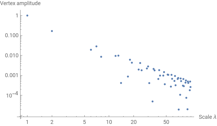
Linear decay in the log-log graph - Power law:
In[]:=
Av=Table[SixJSymbol[{λj,λj,λj},{λj,λj,λj}],{λ,0,100}];Av=Table[{L,Re[Av[[L]]]//N},{L,1,100}];
In[]:=
ListLogLogPlot[Av,AxesLabel->{"Scale λ","Vertex amplitude"},PlotRange->All]
Out[]=
In[]:=
FindFit[Av,ax^b,{a,b},x]
Out[]=
{a1.00254,b-3.14939}
3D Quasicrystalline Spin Foam
3D Quasicrystalline Spin Foam
Consider now a configuration of j's, which give the triangles areas or the volumes of the tetrahedra and give a finite number of them, which can tile 3D Euclidean space in an aperiodic way. Usually quasicrystals will have more complicated tiles or vertex types, but those can be triangulated. Some of the interesting 3D quasicrystals are the ones that have icosahedral symmetry like the three dimensional analogue of the Penrose tiling and the D6 and E8 quasicrystals [5]. Here we explore some polytopes which are building blocks of such quasicrystals. The quasicrystalline spin foam amplitudes in 3D is given from (1), by(QSN[])[j][j] (2)where △ is now the triangulation on top of the quasicrystal, an amplitude for the faces of the dual of △ and the vertex amplitude on the vertices dual of the tetrahedra of △. We can isolate the product over one tiling configuration(QSN[]) (3)with (4)where labels the different tetrahedra vertex types of a given quasicrystal, and are the frequency of the geometric objects times the total number of tiles considered. The spin foam becomes a function of the vertex type frequencies of quasicrystal, which are the important quantities in the descriptions of physics properties of quasicrystals [5]. Lattices and quasicrystals will have precise frequencies while for random structures would be not well defined.
W
△
j
b
N
△
∑
j⊂△
∏
f
A
f
∏
v
A
v
A
f
A
v
W
△
j
b
N
△
∑
j⊂△
A
△
A
△
∏
f
T
n
f
T
j
f
T
(-1)
n
f
T
(2+1)
j
f
∏
v
T
n
V
T
{6j}
v
T
n
f
T
n
V
T
Let us implement the amplitude :
A
△
Let us consider some polytope examples .
Amplitude for the Icosahedron
Amplitude for the Icosahedron
The boundary of the icosahedron is made of regular triangles, we insert a point in the center of the Icosahedron to get tetrahedra
With two half integers we cannot have the precise ratio between the boundary edge length and the bulk edge so we approximate this ratio in the large j limit. The face of the dual complex is dual of a edge of the triangulation such that we can think of the j's being associated with the edge lengths.
We need now the number of faces of the dual. In this case it is simple as the dual is a small dodecahedron inside the icosahedron and so the number of 2-faces are 12 pentagons. The number of vertices of the dual we already have, which is the number of tetrahedra that triangulate the icosahedron - 20.
The SixJSymbol pattern following the integration in [2] is that the first row form a triangle (in this case the regular one) and the lower row has 3 edges coming from the equilateral triangle to the opposite vertex - here the icosahedron center.
The vertex amplitude in this case with 2 spins
Icosahedron Amplitude, and for example the asymptotics:
Amplitude for the Octahedron
Amplitude for the Octahedron
The boundary of the Octahedron is made of regular triangles, we insert a point in the center of the Octahedron to get tetrahedra
The two spins:
The dual:
The vertex amplitude in this case with 2 spins
Octahedron Amplitude, and for example the asymptotics:
4D Quasicrystalline Spin Foam
4D Quasicrystalline Spin Foam
4D Spin Foam
4D Spin Foam
Wigner Generalized 4jm
15j first kind
Boost Matrix Elements for the Simplified Model
The kind of {15 j} that we will use for the 600 - cell has the structure:
And a specific amplitude can be computed:
The use of the simplified model is justified because the sum in the virtual spins converge very fast, using the parallel C code of [9] with γ=1.2 we get:
4D Quasicrystalline Spin Foam
4D Quasicrystalline Spin Foam
The amplitude for the 600-cell
The amplitude for the 600-cell
The procedure is the same as for the icosahedron. We get the information of the 600-cell, insert the center, building 600 golden 4-simplices, then find the dual of this. Basically we need to associate spins to the face of the dual, which are associated to the triangles of the 600-cell plus the triangles in the bulk made with the center, so we need the areas of these triangles too. So let us start by getting the 600-cell from the quasicrystalline project from the E8 lattice.
We are not going on the details of the cut and projection scheme but it selects just one 600-cell from the projection of the E8 roots and we consider the center point, which in fact comes from the E8 Cartans.
Now compute the dual 120-cell
For example, for spins = Permutations[{1, 1, 1, 1, 1, 1, 1, 1, 1, 2, 2, 2, 2, 2, 2}] the non-zero {15j} symbols can be computed:
The amplitudes for one 600 - cell 4 - simplex. They are the same with 4 boundary spins and 6 internal
Each vertex of the the 600-cell has 20 regular tetrahedra (20G) sharing it. It is a building block of the 600-cell. We will discuss more this later but the dual is a dodecahedron and so 12 pentagonal faces. From equation (5) we can compute the amplitude of the 20G in a specific case
Boundary coherent states
Boundary coherent states
Until now the boundary QSN state was specified in general just with the areas of the triangles (the spins j). Now we specify more details, which are the 3D normals of the triangles, then specifying a coherent tetrahedron state [2,6-8]. A coherent tetrahedron is given by:
Then coupling the coherent tetrahedra with the amplitude eq. (5), one for each of the 5 tetrahedra boundary of the 4-simplex.
Twist: Boundary coherent states from Dual Rotations
Twist: Boundary coherent states from Dual Rotations
The problem now is to find the precise angles for our 600-cell observable . We note that fourSimplices600Cell[[540]] has the first tetrahedron in the "time gauge" direction {-1, 0, 0, 0} .
Functions
Functions
◼
To find the dual of a simple rotation in 4D, we find the eigenplane of the rotation, then take its dual plane,
and construct a rotation by the same angle in that dual plane (or allow variable angle).
If the rotation is compound, we find both its eigenplanes, and exchange their rotation angles.
and construct a rotation by the same angle in that dual plane (or allow variable angle).
If the rotation is compound, we find both its eigenplanes, and exchange their rotation angles.
4-simplex
4-simplex
Get the normals of the Desired 4-simplex
Construct the dual rotation
Then compute the 3D normals, first rotate to the same 3D space
Then use the dual rotation to align the normals - reduction of the total number of parallel plane classes, implementing condition (6)
Then Compute the Euler angles. The normals are understood to give a coherent state that was in z axis {0,0,1} direction rotated to the general direction of the normal:
And the 4-simplex amplitude for this particular coherent boundary data observable
In this way phis[[1]] will have the angles for triangle shared by a=1 with b=2...5 for example. The encoding of the connectivity:
with (a,b): j1->(1,2) if in i1 and j1->(2,1) if in i2, and similarly for the others j2->(1,3)or(3,1), j3->(1,4), j4->(1,5), j5->(2,5), j6->(2,4), j7->(2,3), j8->(3,5), j9->(3,4), j10->(4,5) and the same for the thetas:
with (a,b): j1->(1,2) if in i1 and j1->(2,1) if in i2, and similarly for the others j2->(1,3)or(3,1), j3->(1,4), j4->(1,5), j5->(2,5), j6->(2,4), j7->(2,3), j8->(3,5), j9->(3,4), j10->(4,5) and the same for the thetas:
600-Cell
600-Cell
3D concept illustration : Flattening icosahedron faces to edge/vertex/face planes
3D concept illustration : Flattening icosahedron faces to edge/vertex/face planes
The dual connection between hyperplane rotations and twists cannot exist in dimensions less than 4, since those do not support dual rotations.
4D, however, is hard to visualize, and so it is a difficult setting in which to establish the basic concepts that are needed. While not all these concepts have analogs in 3D, many do, and so we begin with 3D examples to illustrate some of the basics: various groups of neighboring faces flattened by rotation to a single plane. With those concepts and terminology established, we will proceed in the next section to the 4D case, where there is a dual rotation (the twist) which is meaningful.
4D, however, is hard to visualize, and so it is a difficult setting in which to establish the basic concepts that are needed. While not all these concepts have analogs in 3D, many do, and so we begin with 3D examples to illustrate some of the basics: various groups of neighboring faces flattened by rotation to a single plane. With those concepts and terminology established, we will proceed in the next section to the 4D case, where there is a dual rotation (the twist) which is meaningful.
◼
Display
600-cell vertex cap 20G (20 tetrahedral facets sharing a single vertex)
600-cell vertex cap 20G (20 tetrahedral facets sharing a single vertex)
For the 20G in the 600-cell the vertex cap is an icosahedron, and its dual dodecahedron is one dodecahedron of the dual 2-complex. Select one vertex to be the pole, sort vertices by distance from pole and get the 3D space normal to that pole to be the target for the common rotation. Rotate each tetrahedron into the target space, flattening the whole vertex cap into 3D, and then twist each tetrahedron by the dual of its flattening rotation.
◼
Define.
◼
Display
20G - Flatten/twist face-to-face sequential
20G - Flatten/twist face-to-face sequential
Let us pick a second vertex from fourSimplices600CellRef, which then is in poleVertex' s vertex cap, and the edge between the poleVertex and vertex 2 will be shared by 5 tets in the cap. We flatten this group as follows:
First rotate tet 5 into the space of tet 4, then rotate tets 5 and 4 into the space of tet 3, and so on until all 5 are in the space of tet 1. The dual of each flattening rotation is a twist.
First rotate tet 5 into the space of tet 4, then rotate tets 5 and 4 into the space of tet 3, and so on until all 5 are in the space of tet 1. The dual of each flattening rotation is a twist.
◼
Display
Coupling fermions in the fundamental representation of SU(3)
Coupling fermions in the fundamental representation of SU(3)
Function to generate a random SU(3) matrix
Function to compute the character for the fundamental representation of SU(3)
Compute the integral with a given number of iterations
The situation is similar for the SL(2,C) U matrices in the fundamental representation. It is interesting to note that the j values are associated to the triangle areas of the tetrahedron dual of the edges. The SL(2,C) group elements of gravity can be in any representation while the fermion is in the 1/2 representation. This indicate that the adding one fermionic family of cycles is adding an additional layer with small areas compared with the large j limit of the gravitational sector. Usually one would consider that the Us and gravitational elements would be the same to couple fermions with gravity and integrate over everything. Here we are keeping the two sector integrations separated. The gravitational amplitude was computed in the previous section.
The state at each tetrahedron is labeled by the coherent state spin network with the spins, intertwiners and normals. Now we add the fermionic Fock space which can be 0 for the vacuum, and if there is a matrix U in the fundamental representation it means there is 2 states labeled by ±1/2 spins. It can have also two cycles or two matrices, in this case the tensor product space with a new quantum number.
We also can associate the SU(3) charge with the volume of the tetrahedron dual of the SU(3) edge. The intertwiner Hilbert spaces grows with the representations but the U layer has specific lower representation, it has fixed volume eigenspace and eigenvalues. Following [2] let us compute the volume eigenvalues. The square of the volume is obtained from:
And we remember that the SU(3) charge in particle physics comes from the weights of the fundamental representation
So it is attempt to map the lowers dimensional intertwiner spaces of the matter layers with the SU(3) charge Hilbert spaces, which the details we will leave as work in progress.
Note on E8 Unification
Note on E8 Unification
So, we can consider that the Hilbert spaces labeled by j in the spin network are coming from E8 representation spaces. The one dimensional lattice given from α is the A1 root lattice embed in higher dimension - the root lattice gives the spin quantum numbers from the root vectors.
We can recover the E8 roots for example:
the regular tetrahedron reference in the {-1,0,0,0} direction
References
References
◼
[1] Amaral, M.; Clawson, R.; Irwin, K. Quasicrystalline Spin Foam with Matter: Definitions and Examples, [arXiv:2306.01964 [gr-qc]]. (2023).
◼
[2] Rovelli, C., Vidotto, F.: Covariant Loop Quantum Gravity. Cambridge University Press 1 edition, (2014).
◼
[3] Amaral, M., Aschheim, R., Irwin, K. Quantum walk on a spin network, arXiv:1602.07653 [hep-th], (2016).
◼
[4] Amaral, M., Aschheim, R., Irwin, K. Quantum gravity at the fifth root of unity. Physics Open, Volume 10, 100098, (2022).
◼
[5] Baake, M., Grimm, U.: Aperiodic Order, Cambridge University Press, (2013).
◼
[6] Speziale, S. Boosting Wigner’s nj-symbols. J. Math. Phys. 58, 032501 (2017). arXiv:1609.01632v2 [gr-qc].
◼
[7] Dona, P., Sarno, G., Numerical methods for EPRL spin foam transition amplitudes and Lorentzian recoupling theory, Gen. Rel. Grav. 50, 127, (2018).
◼
[8] Dona, P., Fanizza, M., Sarno, G., Speziale, S., Numerical study of the Lorentzian Engle-Pereira-Rovelli-Livine spin foam amplitude. Phys. Rev. D 100, 106003 (2019);
◼
[9] Francesco Gozzini, A high-performance code for EPRL spin foam amplitudes. Class. Quantum Grav. 38 225010 (2021).
◼
[10] Elser, V., Sloane, N. J. A., A highly symmetric four-dimensional quasicrystal, J. Phys. A 20, 6161, (1987).
◼
[11] Sadoc, J. F. and Mosseri, R. The E8 lattice and quasicrystals: geometry, number theory and quasicrystals. J. Phys. A: Math. Gen. 26 1789, (1993).
◼
[12] Fang, F.; Clawson, R.; Irwin, K. Closing Gaps in Geometrically Frustrated Symmetric Clusters: Local Equivalence between Discrete Curvature and Twist Transformations. Mathematics 2018, 6, 89.
◼
[13] Fang, F., Irwin, K. An Icosahedral Quasicrystal and E8 derived quasicrystals. arXiv:1511.07786v2 [math.MG]. (2016).
CITE THIS NOTEBOOK
CITE THIS NOTEBOOK
Quasicrystalline spin foam with matter: computations
by Marcelo Amaral and Richard Clawson
Wolfram Community, STAFF PICKS, June 1, 2023
https://community.wolfram.com/groups/-/m/t/2929437
by Marcelo Amaral and Richard Clawson
Wolfram Community, STAFF PICKS, June 1, 2023
https://community.wolfram.com/groups/-/m/t/2929437