State transition diagrams are networks of hypergraphs which show the steady states which each hypergraph tends towards over time. The diagrams usually contain all possible initial conditions of a specific hypergraph signature and then the network shows how each condition changes after applying one specific rule.
For signature-preserving rules, that is rules which don’t generate extra relations, the state transition diagrams should be finite. Hence, they should show the basin of attractors that all the other states tend towards and will eventually end up in.
For example, let’s consider a simple hypergraph signature with a simple rule with signature 2. We first need to generate all the possible initial conditions of that hypergraph signature:
For signature-preserving rules, that is rules which don’t generate extra relations, the state transition diagrams should be finite. Hence, they should show the basin of attractors that all the other states tend towards and will eventually end up in.
For example, let’s consider a simple hypergraph signature
2
2
2
2
In[]:=
AllEnumeration[List_]:=ResourceFunction["EnumerateHypergraphs"][List];
In[]:=
Graph22AllInitials=AllEnumeration[{{2,2}}]
Out[]=
{{{1,1},{1,1}},{{1,1},{1,2}},{{1,1},{2,1}},{{1,2},{1,2}},{{1,2},{2,1}},{{1,2},{1,3}},{{1,2},{2,3}},{{1,2},{3,2}}}
Now, we need to apply the rule to each one of these conditions and form an association of the directed relations between the different hypergraphs:
In[]:=
AllRelations[input_,rule_]:=ResourceFunction["ParallelMapMonitored"][#ResourceFunction["FindCanonicalHypergraph"][Last[ResourceFunction["WolframModel"][rule,#,1,"StatesList"]]]&,input];
In[]:=
Graph22AllRelations=AllRelations[Graph22AllInitials,{{1,2},{2,3}}{{2,1},{3,1}}]
Out[]=
{{{1,1},{1,1}}{{1,1},{1,1}},{{1,1},{1,2}}{{1,1},{2,1}},{{1,1},{2,1}}{{1,2},{1,2}},{{1,2},{1,2}}{{1,2},{1,2}},{{1,2},{2,1}}{{1,1},{2,1}},{{1,2},{1,3}}{{1,2},{1,3}},{{1,2},{2,3}}{{1,2},{3,2}},{{1,2},{3,2}}{{1,2},{3,2}}}
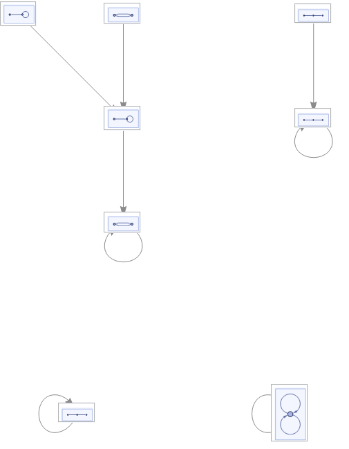
The above is a list of each initial condition and the next state that it evolves to after applying the rule for one time. Note that since we started with all possible initial conditions and we are using a signature-preserving rule, applying the rule one time should produce all possible hypergraphs under that rule and that signature. That should be all we need to produce the state transition diagram:
In[]:=
panelLabel[lbl_]:=Panel[Framed[Style[lbl,Hue[0.62,1,0.48]],BackgroundDirective[{Hue[0.63,0.41,1],Opacity[0.115]}],FrameStyleDirective[Opacity[0.5],Hue[0.62,0.52,0.82]]],FrameMargins0]
In[]:=
StateNetwork[input_]:=Graph[input,VertexLabels((First[#]Placed[ResourceFunction["WolframModelPlot"][First[#],ImageSize20],Center,panelLabel]&/@input)),PerformanceGoal"Quality",EdgeStyleResourceFunction["WolframPhysicsProjectStyleData"]["StatesGraph","EdgeStyle"]]
In[]:=
StateNetwork[Graph22AllRelations]
Out[]=
We can repeat the same steps above with the same rule but this time for hypergraph signature :
3
2
In[]:=
Graph32AllInitials=AllEnumeration[{{3,2}}];Graph32Relations=AllRelations[Graph32AllInitials,{{1,2},{2,3}}{{2,1},{3,1}}];StateNetwork[Graph32Relations]
Out[]=
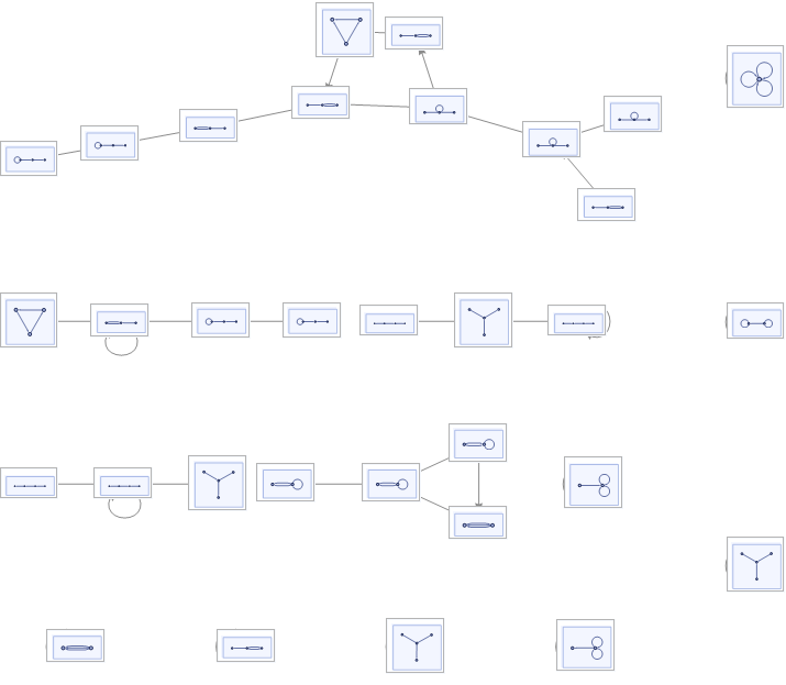
What is very interesting in these networks is that they exhibit the entire phase space of the system under the specific chosen configurations (hypergraph and rule signature). This allows us to see two disjoint sets of hypergraphs: the transient hypergraphs and the attractors. These two sets of hypergraphs are particularly interesting because they can have several interpretations in physics. For example, one can argue that the hypergraphs in the basin of attractors are high entropy states and the transient hypergraphs are low entropy states. This intuition comes from the second law of thermodynamics which says that all the states tend towards high entropy states. So if the law applied to the hypergraphs then the attractor hypergraphs are the high entropy states because these are the states that all the other states in the phase space tend towards.
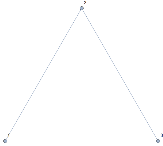
This argument might not be completely valid since entropy is a a property of the ensemble that results by coarse-graining the microstates of the systems, and these hypergraphs are just the microstates. However, we can use that argument to find some graph theoretic properties that can distinguish the transient hypergraphs and the attractor hypergraphs. Since the microstates of the system are hypergraphs, then the best interpretation of their entropy would be Shannon’s entropy or the information entropy. The interpretation of the entropy in this case will be the amount of uncertainty in identifying each constituent of the hypergraph, or in other words, how much information is needed to describe and distinguish each of the nodes in the hypergraph. If the hypergraph has sufficient information that makes each node distinguishable, then it’s a low entropy hypergraph, if no information is contained and the nodes are not distinguishable, then it’s a high entropy hypergraph. For example, let’s consider the following hypergraph from the basin of attractors that we looked at above:
This argument might not be completely valid since entropy is a a property of the ensemble that results by coarse-graining the microstates of the systems, and these hypergraphs are just the microstates. However, we can use that argument to find some graph theoretic properties that can distinguish the transient hypergraphs and the attractor hypergraphs. Since the microstates of the system are hypergraphs, then the best interpretation of their entropy would be Shannon’s entropy or the information entropy. The interpretation of the entropy in this case will be the amount of uncertainty in identifying each constituent of the hypergraph, or in other words, how much information is needed to describe and distinguish each of the nodes in the hypergraph. If the hypergraph has sufficient information that makes each node distinguishable, then it’s a low entropy hypergraph, if no information is contained and the nodes are not distinguishable, then it’s a high entropy hypergraph. For example, let’s consider the following hypergraph from the basin of attractors that we looked at above:
In[]:=
Example1=Graph[{{1,2},{2,3},{3,1}},VertexLabelsAutomatic]
Out[]=
In[]:=
VertexInDegree[Example1,#]&/@VertexList[Example1]
Out[]=
{2,2,2}
This hypergraph is symmetric and isomorphic. This doesn’t give us enough information that would allow us to identify any individual node. All nodes have the same in and out degrees. So if we ignore the labels, then there is no way we can fully describe a node in that hypergraph (e.g. we can’t say the node with two edges because the three nodes have two edges). This means that the uncertainty in that hypergraph is high or, in other words, it’s a high entropy state hypergraph (it doesn’t provide much information about its constituents).
On the other hand, the following hypergraph comes from the transient set of hypergraphs:
On the other hand, the following hypergraph comes from the transient set of hypergraphs:
In[]:=
Example2=Graph[{{1,2},{1,2},{3,1}},VertexLabelsAutomatic]
Out[]=

In[]:=
VertexInDegree[Example2,#]&/@VertexList[Example2]
Out[]=
{3,2,1}
It’s obvious that this hypergraph provides much information about its constituents that makes it easy to identify each one of them. For example, if I say “the node with three edges”, then it will be clear that I’m talking about node 1. Therefore, the uncertainty in that hypergraph is low and hence it’s a low entropy hypergraph.
So using the to examples above, we were able to distinguish between an attractor hypergraph and a transient hypergraph using the vertex transitivity and the hypergraph isomorphism. We can now see if these properties will succeed to distinguish the two types of hypergraphs at high scales. To be able to make some quantification of the difference, we can use the variance of the in-degree of the vertices of each hypergraph. According to the discussion above, the attractors should have similar nodes (symmetric structure) and then the variance of their vertices in-degree should then be lower than that of the transients hypergraphs. Here are the variances for the two examples above:
So using the to examples above, we were able to distinguish between an attractor hypergraph and a transient hypergraph using the vertex transitivity and the hypergraph isomorphism. We can now see if these properties will succeed to distinguish the two types of hypergraphs at high scales. To be able to make some quantification of the difference, we can use the variance of the in-degree of the vertices of each hypergraph. According to the discussion above, the attractors should have similar nodes (symmetric structure) and then the variance of their vertices in-degree should then be lower than that of the transients hypergraphs. Here are the variances for the two examples above:
In[]:=
Variance[VertexInDegree[Example1,#]&/@VertexList[Example1]]
Out[]=
0
In[]:=
Variance[VertexInDegree[Example2,#]&/@VertexList[Example2]]
Out[]=
1
High entropy states have low variance and low entropy states have high variance. So the property that we will be using is the variance of the vertices in - degree in different hypergraphs. Let' s start by writing the functions we need to generate a big set of hypergraphs.
Find Attractors. The following function will find all the hypergraphs in the basin of attraction of the transition diagrams. There are two types of attractors: one that form cycles and one that form self-loops.
In[]:=
FindAttractors[graph_]:=Module[{Loops,Cycles},Loops=DeleteCases[If[Length[VertexOutComponent[graph,#]]1&&VertexInDegree[graph,#]>1,#]&/@VertexList[graph],Null];Cycles=VertexOutComponent[graph,#]&/@VertexList[graph];Cycles=Sort[#]&/@Cycles;Cycles=Cases[Tally@Cycles,{x_,n_/;n>1}x];Cycles=Flatten[Cycles,1];Join[Cycles,Loops]];
Find Transients. The following function will find the transient hypergraphs.
In[]:=
FindTransients[graph_]:=DeleteCases[If[VertexInDegree[graph,#]0,#]&/@VertexList[graph],Null]
Put it all together. The following function puts all the functions above together to generate a list of all the attractors and a list of all the transients inside a state transition diagram.
In[]:=
GenerateGraphs[GraphSize_,rule_]:=Module[{AllEnum,relations},AllEnum=AllEnumeration[{{GraphSize[[1]],GraphSize[[2]]}}];relations=AllRelations[AllEnum,rule];relations]
In[]:=
AppendGraphs[graphsize_,rule_,attrclist_,initlist_]:=Module[{GeneratedGraphs,attractors,initials},GeneratedGraphs=GenerateGraphs[graphsize,rule];attractors=FindAttractors[GeneratedGraphs];initials=FindTransients[GeneratedGraphs];attractors=Union[attrclist,attractors];initials=Union[initlist,initials];attractors=Select[attractors,Not[MemberQ[initials,#]]&];Return[{attractors,initials}]];
Now, we can start generating sets of hypergraphs and see their properties.
We can see that in all the hypergraphs and rules we checked above, the average variance of in-indegree is always lower for the attractors. For example, we can check these histograms for the state transition diagram that we started this post with:
Looking at the two histograms, we see that the variance is much smaller for the attractors than for the transients. This correlation is consistent over several rules and graph signatures. As I mentioned earlier, the characterization of this correlation as being a result of the entropy increase due to the time evolution of hypergraphs is interesting but still might not be completely valid because there still might be a reverse-process that can take the state of the hypergraphs in the attractors backward. However, this strong correlation of the in-degree variance in very interesting and should be examined further.
Excluded Sub-hypergraphs.
Excluded Sub-hypergraphs.
Another interesting thing to look at using these state transition diagrams is the exclusion of sub-hypergraphs during the time evolution of the hypergraphs. It might be the case that after a certain number of steps, certain sub-hypergraphs are excluded. Knowing these sub-hypergraphs is useful because it can tell us that after T steps we can only have hypergraphs that don’t contain these excluded blocks.
To investigate that, I will start a specific hypergraph signature, generate all possible initial condition of that signature and then apply the rules for several steps on all of these conditions. At each step, I will keep track of the sub-hypergraphs that get excluded or included. After T steps, this should tell me whether any block got excluded and when.
To investigate that, I will start a specific hypergraph signature, generate all possible initial condition of that signature and then apply the rules for several steps on all of these conditions. At each step, I will keep track of the sub-hypergraphs that get excluded or included. After T steps, this should tell me whether any block got excluded and when.
After examining each of these subgraphs that get generated at different time steps, I found the following interesting results:
Future Work
Future Work
The correlation that I found between the attractors-transients and in-degree variance is a very interesting emergent property that should be further examined. This correlation might have different interpretations in physics and then it should be checked against some other physical properties to see if any property can provide a meaningful justification for it.
Acknowledgment
Acknowledgment
I would like to thank my mentor Jack Heimrath for his continuous support and help with all the technical details. I would also like to thank Kiel Howe, Jonathan Gorard and Max Piskunov for their help with the project during the summer school.