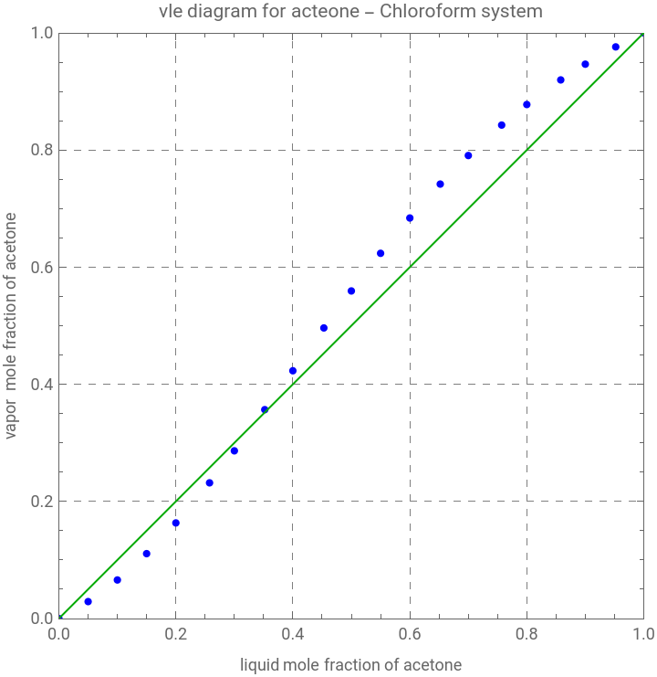
The notebook fits the van Laar activity coefficient model to experimental VLE data for the acetone-chloroform system at atmospheric pressure (14.696 psia) using Particle Swarm Optimization. The script begins with 21 experimental data points of liquid mole fraction, vapor mole fraction, and boiling temperature for acetone, plotted against the y=x reference diagonal. Notably, the experimental curve lies below the diagonal for most of the composition range and crosses it near x ≈ 0.35, which is the signature of a system with negative deviations from Raoult’s law and a maximum-boiling azeotrope — consistent with the known acetone-chloroform system. Vapor pressures for each pure component are computed using the Antoine equation in a slightly different form.
The core equilibrium model again uses the Van Laar activity coefficient equations (gamma1, gamma2) combined with modified Raoult’s law in the myvle function, which solves for vapor composition and temperature at each liquid composition point using FindRoot. Before running the optimizer, the code includes a useful validation step: it manually sets A12 = -0.864 and A21 = -0.5889 — values taken directly from literature — and evaluates the Fitness function, getting a very small loss of 1.83×10⁻⁸. This serves as a check/benchmark to confirm that these literature-reported parameters essentially perfectly reproduce the experimental dataset, and notably, both parameters are negative, which is required to model the negative deviation behavior of this system (unlike the positive-deviation ethanol-water case).
The same custom PSO algorithm is then used, with search bounds tightened to [-2, 1] to allow the optimizer to explore negative parameter space. Running 500 particles for 100 iterations, the loss drops rapidly from 0.068 (iteration 10) to ~1.83×10⁻⁸ by iteration 70, where it plateaus — and the optimizer converges to A12 = -0.864, A21 = -0.5889, exactly matching the literature benchmark values tested earlier. This confirms the PSO implementation is correctly identifying the global optimum rather than getting stuck in a local minimum. The final fitted curve (red) is overlaid on the experimental data (blue points) and the y=x diagonal (green), showing the model accurately captures the S-shaped curve and the azeotropic crossing point near 0.35 mole percent acetone.
Acetone-Chloroform VLE Data at 1 atm
Columns:X_Acetone (liquid),Y_Acetone (vapor),T (°C)
Columns:X_Acetone (liquid),Y_Acetone (vapor),T (°C)
vleData={{0.,0.,61.1789},{0.05,0.0289316,61.9318},{0.1,0.0658663,62.6542},{0.15,0.110809,63.2994},{0.2,0.163269,63.8287},{0.2576,0.231719,64.2576},{0.3,0.286385,64.434},{0.352,0.356683,64.4819},{0.4,0.423096,64.3634},{0.453,0.496198,64.0625},{0.5,0.559372,63.6619},{0.55,0.623636,63.1175},{0.6,0.68395,62.4734},{0.652,0.741836,61.7219},{0.7,0.790595,60.975},{0.757,0.842596,60.046},{0.8,0.877692,59.3292},{0.858,0.919713,58.358},{0.9,0.946593,57.6609},{0.952,0.976108,56.8139},{1.,1.,56.0544}};
Extract columns
xAcet=vleData[[All,1]];yAcet=vleData[[All,2]];tempC=vleData[[All,3]];
Plot Psat vs T
plt1=ListPlot[Transpose@{xAcet,yAcet},PlotStyle->{Blue,Thick},Frame->True,FrameLabel->{"liquid mole fraction of acetone","vapor mole fraction of acetone"},PlotLabel->"vle diagram for acteone - Chloroform system",GridLines->Automatic,GridLinesStyle->Directive[Gray,Dashed],AspectRatio->1,PlotRange->{{0,1},{0,1}},Epilog->{Darker@Green,Line[{{0,0},{1,1}}]}]
Out[]=
In[]:=
P=14.696;
Antoine Equation where Temperature in °C and Pressure in mmHg
Aa1=6.244412;Ba1=5356.715;Ca1=397.5290;Aa2=5.894057;Ba2=5289.385;Ca2=393.075;Psat1[t_]:=693.7E^(Aa1-Ba1/((t)1.8+32+Ca1));(*Acetone*)Psat2[t_]:=793.6E^(Aa2-Ba2/((t)1.8+32+Ca2));(*Chloroform*)
In[]:=
FindRoot[Psat1[t]==P,{t,58}]
Out[]=
{t56.0544}
In[]:=
FindRoot[Psat2[t]==P,{t,58}]
Out[]=
{t61.1789}
In[]:=
Length@tempC
Out[]=
21
In[]:=
Length@xAcet
Out[]=
21
Van Laar Model
gamma1[A12_,A21_,x_]:=Exp[A12(A21(1-x)/(A12x+A21(1-x)))^2];gamma2[A12_,A21_,x_]:=Exp[A21(A12x/(A12x+A21(1-x)))^2];
In[]:=
myvle[A12_,A21_]:=Module[{i,system,sol,x,t,y},(*Systemofequationsforxandydetermination*)system[x_]:={Py==gamma1[A12,A21,x]*Psat1[t]x,gamma1[A12,A21,x]*Psat1[t]x+gamma2[A12,A21,x]*Psat2[t](1-x)==P};i=1;While[i<=21,{x=xAcet[[i]];sol[i]=Quiet@FindRoot[system[x],{t,60},{y,0.5},MaxIterations->1000];i++}];Table[{y,t}/.sol[i],{i,1,21}]]
In[]:=
SwarmDim=2;(*3Dproblem*)(*upperandlowerboundsfothesearchdomain*)FitnessLB=-2;FitnessUB=1;c1=1.42;c2=1.42;w=0.72984;(*psoparameters*)Fitness[{A12_,A21_}]:=Module[{tbl},tbl=myvle[A12,A21];Sum[(tbl[[i]][[1]]-yAcet[[i]])^2+(tbl[[i]][[2]]-tempC[[i]])^2,{i,1,Length@tempC}]]
In[]:=
Clear[A12,A21]
In[]:=
A12=-0.864;A21=-0.5889;
In[]:=
Fitness[{A12,A21}]
Out[]=
1.8323×
-8
10
In[]:=
Clear[A12,A21]
PSO Optimizer
psoOptimize[lossFunc_,dim_,lb_,ub_,nParticles_:500,nIter_:50,w_:0.72984,c1_:2,c2_:2]:=Module[{particles,velocities,pbest,pbestScore,gbest,gbestScore,convergence={},r1,r2,score,gbestIdx},(*Initializeparticlesuniformlywithin[lb,ub]ineachdimension*)particles=RandomReal[{lb,ub},{nParticles,dim}];velocities=ConstantArray[0.,{nParticles,dim}];pbest=particles;pbestScore=Table[lossFunc[particles[[i]]],{i,nParticles}];gbestIdx=First@Ordering[pbestScore,1];gbestScore=pbestScore[[gbestIdx]];gbest=pbest[[gbestIdx]];Do[Do[r1=RandomReal[1,dim];r2=RandomReal[1,dim];velocities[[i]]=w*velocities[[i]]+c1*r1*(pbest[[i]]-particles[[i]])+c2*r2*(gbest-particles[[i]]);particles[[i]]+=velocities[[i]];(*keepparticleswithinbounds*)particles[[i]]=Clip[particles[[i]],{lb,ub}];score=lossFunc[particles[[i]]];If[score<pbestScore[[i]],pbest[[i]]=particles[[i]];pbestScore[[i]]=score;];,{i,nParticles}];gbestIdx=First@Ordering[pbestScore,1];gbestScore=pbestScore[[gbestIdx]];gbest=pbest[[gbestIdx]];AppendTo[convergence,gbestScore];If[Mod[t,10]==0,Print["PSO Iter ",t," Loss = ",gbestScore]];,{t,nIter}];{gbest,gbestScore,convergence}];
Run PSO
{bestPos,bestScore,convergence}=psoOptimize[Fitness,SwarmDim,FitnessLB,FitnessUB,50,100,w,c1,c2];Print["Best position: ",bestPos];Print["Best fitness: ",bestScore];
PSO Iter 10 Loss = 0.0682788
PSO Iter 20 Loss = 0.00323075
PSO Iter 30 Loss = 0.0000303407
PSO Iter 40 Loss = 1.26721×
-6
10
PSO Iter 50 Loss = 2.47141×
-7
10
PSO Iter 60 Loss = 2.07246×
-7
10
PSO Iter 70 Loss = 1.88167×
-8
10
PSO Iter 80 Loss = 1.88167×
-8
10
PSO Iter 90 Loss = 1.8274×
-8
10
PSO Iter 100 Loss = 1.8274×
-8
10
Best position: {-0.864,-0.5889}
Best fitness: 1.8274×
-8
10
Best position = {-0.864,-0.5889}
In[]:=
A12=-0.864;A21=-0.5889;(*binaryinteractionparametersfromlitterature*)Fitness[{A12,A21}]
Out[]=
1.8323×
-8
10
CITE THIS NOTEBOOK
CITE THIS NOTEBOOK
van Laar equation parameters for acetone - chloroform system via particle swarm optimization
by Housam Binous
Wolfram Community, STAFF PICKS, June 29, 2026
https://community.wolfram.com/groups/-/m/t/3740729
by Housam Binous
Wolfram Community, STAFF PICKS, June 29, 2026
https://community.wolfram.com/groups/-/m/t/3740729