ABSTRACT (original article): The degree of experimentally attainable nonlocality, as gauged by the amount of loophole-free violation of Bell inequalities, remains severely limited due to inefficient detectors. We address an experimentally motivated question: Which quantum strategies attain the maximal loophole-free nonlocality in the presence of inefficient detectors? For any Bell inequality and any specification of detection efficiencies, the optimal strategies are those that maximally violate a tilted version of the Bell inequality in ideal conditions. In the simplest scenario, we demonstrate that the quantum strategies that maximally violate the tilted versions of Clauser-Horne-Shimony-Holt inequality are unique up to local isometries. However, self-testing via the standard sum of squares decomposition method turns out to be analytically intractable since even high levels of the Navascués--Pironio--Acín hierarchy are insufficient to saturate the maximum quantum violation of these inequalities. Instead, we utilize a novel Jordan’s lemma-based proof technique to obtain robust analytical self-testing statements for the entire family of tilted-Bell inequalities. These results allow us to unveil intriguing aspects of the effect of inefficient detectors and the complexity of characterizing the set of quantum correlations, in the simplest Bell scenario. CITATION (original article): N. Gigena, E. Panwar, G. Scala, M. Araujo, M. Farkas, and A. Chaturvedi, Robust self-testing of Bell inequalities tilted for maximal loophole-free nonlocality, arXiv:2405.08743. https://doi.org/10.48550/arXiv.2405.08743
In this computational essay we want to guide the reader through the self-testing of doubly tilted CHSH. Self-testing is a powerful method used in quantum information theory that allows one to verify the realization, also known as 'quantum strategy' (state and measurements) of a quantum system based solely on the observed statistics of the system, without any prior knowledge of the inner workings of the devices involved nor the dimensionality of the Hilbert spaces involved. This is particularly useful in quantum cryptography, where the goal is to establish secure communication between two parties while protecting against eavesdropping or tampering.This supplementary materials is structured as follows: Given → =(analogously for β) the parameters related to the inefficiency of the detectors, - Analysis for α=β -Analisis for α≠β,
α=(1-)
2
η
a
η
a
η
a
2
2+α
0. Elementary Settings (remember to activate MaTeX for plots)
0. Elementary Settings (remember to activate MaTeX for plots)
In this section we setup MaTeX for graph labels
L
A
TE
X(*uncommentifyouneedtoinstallMaTeXResourceFunction["MaTeXInstall"][]*)
Out[]=
PacletObject


In[]:=
ConfigureMaTeX["pdfLaTeX"->"C:\\texlive\\2022\\bin\\win32\\pdflatex.exe","Ghostscript"->"C:\\Program Files\\gs\\gs10.00.0\\bin\\gswin64c.exe"]
Out[]=
{CacheSize100,WorkingDirectoryAutomatic,pdfLaTeXC:\texlive\2022\bin\win32\pdflatex.exe,GhostscriptC:\Program Files\gs\gs10.00.0\bin\gswin64c.exe}
(*Typicallyitisenoughtoclickonlyonthefollowinginput*)
In[]:=
<<MaTeX`
In[]:=
(*----------commondroutines------------*)savefiles1[namevariable_,nametxt_]:=Module[{fname,xFile},fname=FileNameJoin[{SetDirectory[NotebookDirectory[]],nametxt}];xFile=OpenWrite[fname];Write[xFile,namevariable];Close[xFile];]readlist[name_]:=Flatten[ReadList[name],1]
1. Definitions - CHSH-Bell Operator via Jordan's lemma
1. Definitions - CHSH-Bell Operator via Jordan's lemma
In this section we define tilted CHSH-Bell inequality for selftesting.(p)=〈〉+α〈〉+β〈〉<=2+α+β.According to the Jordan's lemma The only parameters that define the Alice and Bob settings respectively are and b==.
α,β
1
∑
x=0
1
∑
y=0
xy
(-1)
A
x
B
y
A
0
B
0
a==
cosθ
A
c
A
cosθ
B
c
B
In[]:=
σ
i_
M
i_
|
1
∑
x0=0
1
∑
y0=0
x0y0
(-1)
M
x0
M
y0
σ
3
σ
0
σ
0
σ
3
∂
a
∂
b
RootsGPoly[k,x1,x2,β] computes the roots of the polynomial via the Groebner basis eliminating x1 and x2 on the polynomials obtained by solving a Lagrangian multiplier problem.
p(k)=(α,β)
deg
∑
i=0
c
i
i
k
In[]:=
FullSimplify@MatrixForm/@{[a,b,α,β],[a,b,α],FullSimplify[[Cos[θ],Cos[θ],α]]}
2. Equal inefficiency detectors α=β
2. Equal inefficiency detectors α=β
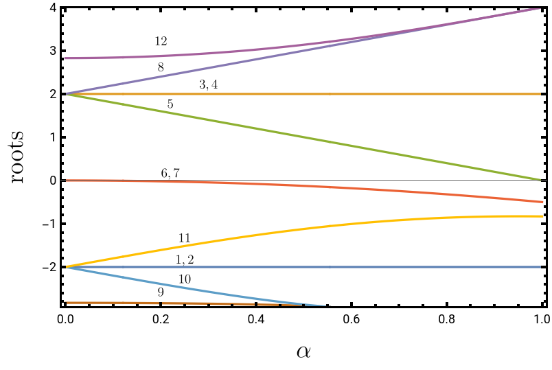
RootsGPoly[k_,x1_,x2_] computes the roots of the polynomial via the Groebner basis eliminating x1 and x2 on the polynomials obtained by solving a Lagrangian multiplier problem. In this way we compute:- optimal quantum value oqv for RootsGPoly[λ,a,b] eliminating a and b. The polynomial is with deg = 12 and the 12th root is the largest;- optimal Alice's settings oAs by eliminating λ and b the polynomial is with deg = 11; - optimal Bob's settings oBs=oAs by eliminating λ and a the polynomial is with deg = 11; We observe that therefore we compute only the optimal Alice setting as the Bob's one coincide.However can be obtained without Groebner basis by the functions oAs(optimal Alice settings) and oAsett (which is a redefinitions of oAs).As the eigenvalues on the optimal realization are non-degenerate the quantum state being related eigenvector to the largest eigenvalue is also self-tested.
p(k)=(α)
deg
∑
i=0
c
i
i
k
p(λ)=(α)
deg
∑
i=0
c
i
i
λ
RootsGPoly[a,λ,b]=p(a)=(α)
deg
∑
i=0
c
i
i
a
RootsGPoly[b,λ,a]=p(b)=(α)
deg
∑
i=0
c
i
i
b
p(a)=p(b)
p(a)
2.1 Optimal quantum value cQ
2.1 Optimal quantum value
c
Q
via the Groebner basis
via the Groebner basis
We compute the optimal quantum value oqv[[12]] as the root of corresponding to the largest.In the following plot all the roots are enumerated.
th
12
p(λ)=(α)
12
∑
i=0
c
i
i
λ
In[]:=
Clear[b]
In[]:=
oqv=RootsGPoly[λ,a,b];oqv[[1]]==oqv[[2]]&&oqv[[3]]==oqv[[4]]&&oqv[[6]]==oqv[[7]]Plot[{oqv[[1]],oqv[[3]],oqv[[5]],oqv[[6]],oqv[[8]],oqv[[9]],oqv[[10]],oqv[[11]],oqv[[12]]},{α,0,1},PlotRange->All,FrameTrue,BaseStyle->{FontFamily->"Times",FontSize->15},PlotRangePadding->0.01,Frame->{{True,False},{True,False}},FrameStyleDirective[Black,Thickness[.004]],FrameTicksStyleDirective[Black,Thick],FrameLabel{MaTeX["\\alpha",Magnification1.5],MaTeX["\\mathrm{roots}",Magnification1.5]},Epilog{Text[MaTeX["12","Preamble"->{"\\usepackage{bm}"},Magnification0.8],{0.2,3.2}],Text[MaTeX["11","Preamble"->{"\\usepackage{bm}"},Magnification0.8],{0.25,-1.35}],Text[MaTeX["10","Preamble"->{"\\usepackage{bm}"},Magnification0.8],{0.25,-2.3}],Text[MaTeX["9","Preamble"->{"\\usepackage{bm}"},Magnification0.8],{0.2,-2.6}],Text[MaTeX["8","Preamble"->{"\\usepackage{bm}"},Magnification0.8],{0.2,2.6}],Text[MaTeX["6,7","Preamble"->{"\\usepackage{bm}"},Magnification0.8],{0.22,.15}],Text[MaTeX["5","Preamble"->{"\\usepackage{bm}"},Magnification0.8],{0.22,1.75}],Text[MaTeX["3,4","Preamble"->{"\\usepackage{bm}"},Magnification0.8],{0.3,2.2}],Text[MaTeX["1,2","Preamble"->{"\\usepackage{bm}"},Magnification0.8],{0.25,-1.85}]}]
Out[]=
True
Out[]=
via the spectrum of [*a(α),*a(α),α,α] with optimal *a (without Groebner basis)
via the spectrum of with optimal (without Groebner basis)
[(α),(α),α,α]
*
a
*
a
*
a
2.2 Optimal Alice=Bob settings
2.2 Optimal Alice=Bob settings
With the Groebner basis (we do not use this approach)
With the Groebner basis (we do not use this approach)
Without the Groebner basis (we use this approach)
Without the Groebner basis (we use this approach)
The following plot takes into account the optimal quantum value.
2.3 Comparison between ideal and noisy CHSH
2.3 Comparison between ideal and noisy CHSH
3. Not equal inefficiency detectors α≠β
3. Not equal inefficiency detectors α≠β
3.2 optimal Alice & Bob settings
3.2 optimal Alice & Bob settings
via Groebner basis
via Groebner basis
All these plot will be shown at the end of the project
3.4 Optimal quantum state and Measure of Entanglement
3.4 Optimal quantum state and Measure of Entanglement
3.4.2 Reading
3.4.2 Reading
Now we read the file and we compute something about the optimal state. pt apply the partial transposition
5. Main figure
5. Main figure
Caption: Optimal quantum value (On the top-left), Schmidt coefficient (on the bottom-left) and optimal settings
CITE THIS NOTEBOOK
CITE THIS NOTEBOOK
Robust self-testing of Bell inequalities tilted for maximal loophole-free nonlocality
by N. Gigena, E. Panwar, G. Scala, M. Araujo, M. Farkas, and A. Chaturvedi
Wolfram Community, STAFF PICKS, July 19, 2024
https://community.wolfram.com/groups/-/m/t/3227123
by N. Gigena, E. Panwar, G. Scala, M. Araujo, M. Farkas, and A. Chaturvedi
Wolfram Community, STAFF PICKS, July 19, 2024
https://community.wolfram.com/groups/-/m/t/3227123