Markov chains represent a fundamental class of probabilistic models capable of describing complex stochastic processes evolving over time. Despite their structural simplicity—grounded in the memoryless property where future transitions depend solely on the current state—they offer a remarkably powerful framework for analyzing dynamic systems. A classic and illustrative application of these models is the random walk on a finite network, particularly within a maze topology.
In this context, the random walk inside a maze can be formalized as a discrete-time random phenomenon. The system consists of a set of discrete states representing the individual cells of the maze grid. At each time step, an agent located at a given state transitions to an adjacent cell, provided that no physical wall obstructs the path. Given that the probability of moving to any neighboring cell depends exclusively on the current position and the topology of accessible neighbors—without regard to the history of previously visited cells—this phenomenon naturally fulfills the Markov property and can be fully modeled by a discrete-time Markov chain.
To rigorously study and simulate this random behavior computationally, two essential tools become necessary:
◼
A graphical visualization routine capable of dynamically generating, modifying, and labeling the maze structure while highlighting the current state of the process during its evolution.
◼
An automated transition matrix builder that programmatically inspects the internal walls and boundary conditions of any given maze topology to construct the corresponding stochastic transition matrix .
Π
The present computational essay explores the mathematical formulation of this random process and details the implementation of these specialized functions in the Wolfram Language, demonstrating how custom algorithmic tools facilitate both the theoretical analysis and the dynamic simulation of Markovian random walks.
Generation of maze and transition matrix
Generation of maze and transition matrix
To analyze a random walk on a maze, it is essential to establish a computational bridge between the geometric representation of the enviroment and its corresponding sthocastic model. In a discrete-time Markov chain, the transition matrix completely dictates the system dynamics, where denotes the probability of moving from cell to cell in a single step. In a maze setting, these probabilities determined by the spacial layout of accessible adjacent cells and the presence of physical barriers.
Π=()
p
i,j
p
i,j
i
j
Manually constructing for arbitrary maze becomes impractical as the dimension grows, or then walls are dynamically added or removed. To overcome this limitation and enable scalable simulations, we developed two core functions in the Wolfram Language:
Π
n
1
.DynamicRandomMaze[n, opts]: Generates an maze topology, supporting custom modifications such as removing or adding specific internal and boundary walls (RemoveWalls, AddWalls), labeling cells (LabelCells), and highlighting the current state (CurrentCell).
n×n
2
.MazeTransitionMatrix[n, opts]: Programmatically inspects the resulting maze layout to build the exact × transition matrix Π automatically identifying absorbing states created by openings on the outer perimeter.
2
n
2
n
To generate the base maze topology, we incorporate ResourceFunction["RandomMaze"], developed by Cong Guo and published in the Wolfram Function Repository . Building upon this baseline architecture, our custom DynamicRandomMaze function extends its functionality by allowing dynamic wall manipulation (removal/addition) and real - time state visualization for the underlying Markov process .
Below, we present the code implementations along with examples illustrating how both functions operate together to construct the stochastic environment .
In[]:=
(*Note:BasetopologygeneratedusingCongGuo'sResourceFunction["RandomMaze"]*)DynamicRandomMaze::usage="DynamicRandomMaze[n] extends ResourceFunction[\"RandomMaze\"] (Guo, C.) by adding wall modification and state highlighting capability for Markov processes.";LabelCells::usage="LabelCells -> True o False indica si se deben numerar las celdas del laberinto.";RemoveWalls::usage="RemoveWalls -> {{cell1, dir1}, {cell2, dir2}, ...} remove the specified walls.";AddWalls::usage="AddWalls -> {{cell1, dir1}, {cell2, dir2}, ...} add the specified walls.";CurrentCell::usage="CurrentCell -> cell or CurrentCell -> (cell -> color) highlights the cell specified as the current state.";Options[DynamicRandomMaze]=Join[Options[ResourceFunction["RandomMaze"]],Options[Graphics],{LabelCells->False,RemoveWalls->{},AddWalls->{},CurrentCell->None}];DynamicRandomMaze[n_Integer,opts:OptionsPattern[]]:=Module[{maze,centros,states,getWallPoints,applyRemove,applyAdd,remWalls,addWalls,labelOpt,currentOpt,currentCellNum,currentColor,mazeOpts,graphicsOpts,mGraphics,getCellGraphics},(*Filterandseparateoptions*)remWalls=OptionValue[RemoveWalls];addWalls=OptionValue[AddWalls];labelOpt=OptionValue[LabelCells];currentOpt=OptionValue[CurrentCell];(*ProcessoptionCurrentCell*){currentCellNum,currentColor}=Replace[currentOpt,{(c_Integer->col_):>{c,col},{c_Integer,col_}:>{c,col},c_Integer:>{c,Orange},_:>{None,Automatic}}];mazeOpts=Sequence@@FilterRules[{opts},Options[ResourceFunction["RandomMaze"]]];graphicsOpts=Sequence@@FilterRules[{opts},Options[Graphics]];(*Generatebasemaze*)maze=ResourceFunction["RandomMaze"][n,mazeOpts];(*Auxiliarystructures*)centros=Transpose[Reverse/@Table[{i,j},{i,1.5,n+0.5,1},{j,1.5,n+0.5,1}]];states=Table[j+n(i-1),{i,1,n},{j,1,n}];(*Obtainthe2ordered(end)pointsofagivenwall*)getWallPoints[s_Integer,direction_String]:=Module[{pos,center,pts},pos=First[Position[states,s]];center=centros[[Sequence@@pos]];pts=Which[direction=="Right",{center+{0.5,-0.5},center+{0.5,0.5}},direction=="Left",{center+{-0.5,-0.5},center+{-0.5,0.5}},direction=="Above",{center+{-0.5,0.5},center+{0.5,0.5}},direction=="Bottom",{center+{-0.5,-0.5},center+{0.5,-0.5}},True,{}];Sort[Round/@pts]];(*Functionsforremovingandaddingwalls*)applyRemove[m_,{s_,dir_String}]:=Module[{targetPts},targetPts=getWallPoints[s,dir];If[targetPts==={},Return[m]];m/.Line[pts_List]/;Sort[Round/@pts]===targetPts:>Sequence[]];applyAdd[m_,{s_,dir_String}]:=Module[{targetPts},targetPts=getWallPoints[s,dir];If[targetPts==={},Return[m]];m/.{Null,lines___}:>{Null,lines,Line[targetPts]}];(*Applywallmodifications*)maze=Fold[applyRemove,maze,remWalls];maze=Fold[applyAdd,maze,addWalls];(*Optionallabelingandcurrentcellhighlighting*)If[TrueQ[labelOpt]||IntegerQ[currentCellNum],getCellGraphics[i_,j_]:=Module[{s,center,isCurrent,bgCol,textCol},s=states[[i,j]];center=centros[[i,j]];isCurrent=(s===currentCellNum);bgCol=If[isCurrent,currentColor,GrayLevel[0.8]];textCol=If[isCurrent,White,Black];{(*Solidfillifitisthecurrentcell*)If[isCurrent,{currentColor,Disk[center,0.315]},Nothing],(*boundaryofthecircle*)If[isCurrent,{Darker[currentColor],Thick},GrayLevel[0.8]],Circle[center,0.315],(*Textofcell*)If[TrueQ[labelOpt],{textCol,Text[Style[s,Bold],center]},Nothing]}];mGraphics=Flatten[Table[getCellGraphics[i,j],{i,1,n},{j,1,n}],1];Show[maze,Graphics[mGraphics],graphicsOpts],Show[maze,graphicsOpts]]]
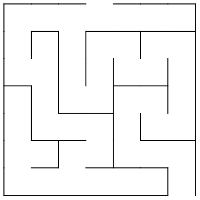
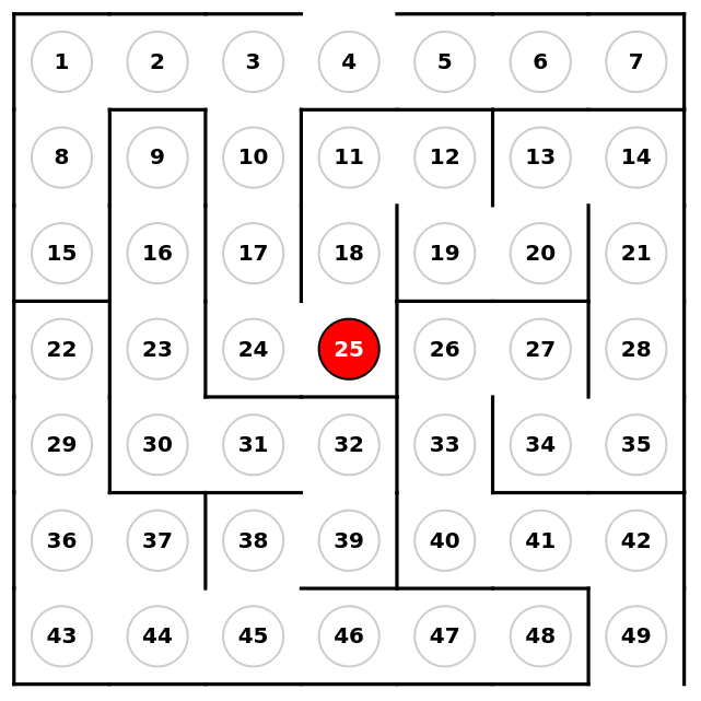
As an example of the use of DynamicRandomMaze, consider the following maze of size and its customized version:
7×7
In[]:=
{SeedRandom["b"];DynamicRandomMaze[7],SeedRandom["b"];DynamicRandomMaze[7,LabelCells->True,CurrentCell->(25->Red),RemoveWalls->{{37,"Bottom"}},AddWalls->{{16,"Left"}}]}
Out[]=
,
In[]:=
MazeTransitionMatrix::usage="MazeTransitionMatrix[n, opts] quickly calculates the transition matrix by identifying absorbing states on the outer boundary.";Options[MazeTransitionMatrix]=Options[DynamicRandomMaze];MazeTransitionMatrix[n_Integer,opts:OptionsPattern[]]:=Module[{mazeGraphic,centros,states,remWalls,addWalls,wallSet,nStates,gridToState,stateToGrid,getWallKey,isWall,isBoundaryWall,absorbingStates,neighbors,transitionRules},remWalls=OptionValue[RemoveWalls];addWalls=OptionValue[AddWalls];nStates=n^2;(*GeneratethegraphicalrepresentationofthemazewithDynamicRandomMaze*)mazeGraphic=DynamicRandomMaze[n,RemoveWalls->remWalls,AddWalls->addWalls,LabelCells->False];(*ExtractwallsandcreateO(1)HashSetforinstantlookups*)wallSet=AssociationThread[Cases[mazeGraphic,Line[pts_List]:>Sort[Round/@pts],Infinity]->True];(*conversionbetweenstatesandgridcoordinates(r,c)*)gridToState[r_Integer,c_Integer]:=c+n(r-1);stateToGrid[s_Integer]:={Quotient[s-1,n]+1,Mod[s-1,n]+1};(*Calculationoftheinternaldividingwallbetweentwoadjacentcells*)getWallKey[r1_,c1_,r2_,c2_]:=Module[{x1,y1,x2,y2,mx,my},{x1,y1}={c1+0.5,(n-r1+1)+0.5};{x2,y2}={c2+0.5,(n-r2+1)+0.5};mx=(x1+x2)/2.;my=(y1+y2)/2.;If[r1==r2,Sort[Round/@{{mx,my-0.5},{mx,my+0.5}}],Sort[Round/@{{mx-0.5,my},{mx+0.5,my}}]]];isWall[r1_,c1_,r2_,c2_]:=KeyExistsQ[wallSet,getWallKey[r1,c1,r2,c2]];(*Wallverificationattheouterborder*)isBoundaryWall[s_Integer,dir_String]:=Module[{r,c,x,y},{r,c}=stateToGrid[s];{x,y}={c+0.5,(n-r+1)+0.5};KeyExistsQ[wallSet,Which[dir=="Above",Sort[Round/@{{x-0.5,y+0.5},{x+0.5,y+0.5}}],dir=="Bottom",Sort[Round/@{{x-0.5,y-0.5},{x+0.5,y-0.5}}],dir=="Left",Sort[Round/@{{x-0.5,y-0.5},{x-0.5,y+0.5}}],dir=="Right",Sort[Round/@{{x+0.5,y-0.5},{x+0.5,y+0.5}}]]]];(*Automaticallydetectabsorbentstatesatopenedges*)absorbingStates=Select[Range[nStates],Function[s,Module[{r,c},{r,c}=stateToGrid[s];(r==1&&!isBoundaryWall[s,"Above"])||(r==n&&!isBoundaryWall[s,"Bottom"])||(c==1&&!isBoundaryWall[s,"Left"])||(c==n&&!isBoundaryWall[s,"Right"])]]];(*Neighborsaccessibletotransitivestates*)neighbors[s_Integer]:=Module[{r,c,cand,validCand},{r,c}=stateToGrid[s];cand={{r-1,c},{r+1,c},{r,c-1},{r,c+1}};validCand=Select[cand,1<=#[[1]]<=n&&1<=#[[2]]<=n&];gridToState@@@Select[validCand,!isWall[r,c,#[[1]],#[[2]]]&]];(*Constructthetransitionmatrix*)transitionRules=Flatten[Table[If[MemberQ[absorbingStates,s],{s,s}->1.,Module[{acc=neighbors[s]},If[Length[acc]>0,Table[{s,dest}->1./Length[acc],{dest,acc}],{s,s}->1.]]],{s,1,nStates}]];Normal[SparseArray[transitionRules,{nStates,nStates}]]]
Visualize the process as a graph:
Simulation
Simulation
Linear system for absorption probabilities
Linear system for absorption probabilities
The vector of absorbing probabilities satisfies the system of linear equations:
subject to the boundary conditions:
Linear System for Mean Absorption Time
Linear System for Mean Absorption Time
In addition to evaluating absorption probabilities, another fundamental property of absorbing Markov chains is the expected time (or mean number of steps) required for a random walk to reach an exit.
By applying first-step analysis (the Law of Total Expectation conditioned on the first transition), $h_A(k)$ satisfies the linear system:
subject to the boundary conditions:
References
References
[1] Norris, J. R. (1997). Markov Chains. Cambridge University Press.
[2] Guo, C. (2019). RandomMaze. Wolfram Function Repository. https://resources.wolframcloud.com/FunctionRepository/resources/RandomMaze/
[3] Google. (2026). Gemini (July 2026 version) [Large language model]. https://gemini.google.com/
AI Tool Usage Declaration:
During the preparation of this work, the author used Google Gemini for stylistic and grammatical refinement of the text, as well as for code optimization and structuring in Wolfram Language. Following the generation of AI-suggested content, the author reviewed, validated, and accepted full responsibility for the final content presented.
During the preparation of this work, the author used Google Gemini for stylistic and grammatical refinement of the text, as well as for code optimization and structuring in Wolfram Language. Following the generation of AI-suggested content, the author reviewed, validated, and accepted full responsibility for the final content presented.
CITE THIS NOTEBOOK
CITE THIS NOTEBOOK
Modeling random walks on mazes via discrete Markov chains
by Diego Ramos
Wolfram Community, STAFF PICKS, July 26, 2026
https://community.wolfram.com/groups/-/m/t/3767968
by Diego Ramos
Wolfram Community, STAFF PICKS, July 26, 2026
https://community.wolfram.com/groups/-/m/t/3767968