What is Chaos?
What is Chaos?
These days it’s become more difficult to appreciate the word “chaos” for what it was originally intended to mean. Distressing worldly conditions have drawn our attention toward disaster and calamity, and away from etymology and deep history. Ancient sages didn’t have a scientific picture of the “primordial fireball” giving rise to the observable universe, so they ended up mostly spinning colorful yarns about where we came from and what the world is made of. In these old stories, Chaos is said to be the murky, formless, generative predecessor of the clear and sharply defined world as we know it today.
When venturing out around earth, we humans also became captivated by its natural beauty, and pursued order as a means to escape our own chaotic ignorance. Not only did we discover pearls, opals, jade, beryls, rubies, sapphires, diamonds, other gems and precious metals, we also learned about circles, lines, squares, cubes, polyhedra, tilings, spheres, and crystal lattices. It’s always rewarding and enjoyable to look closely and find beauty where least expected. Finding order from chaos is again our goal here.
In this era of computation, scientists have seized upon the omnipotential aspect of chaos by defining that chaotic functions should behave in an unpredictable way, especially with regard to perturbations of their initial conditions. The recent movement roughly started with Lorenz’s discovery of the butterfly attractor, a wonderful image of order produced from a continuous chaotic function. Although Stephen Wolfram's latest blog has a nice section on continuous functions, we’ve lately looked more closely at discrete functions such as the "nested recursive P312" function. As recounts the blog, candidate P312 turned out to be a red herring in its ultimate reducibility. This was a momentary disappointment leading us to look elsewhere for a set of functions with genuinely unexpected behavior.
After some amount of trial and error, we finally found interest in a family of functions closely related to the Hofstadter G-Sequence. A few examples included in the blog already show the mixing of chaos and order, but there are still many more results to uncover. We will delineate a graded search space with infinitely many levels. By exhaustive searching through lowest lying levels, we will show that among thousands of viable alternatives, a very few particular functions stand out as special and unique with regard to a randomness test on the distribution of even and odd numbers. These “Missing Gems” function are wonders producing order from chaos. If anyone else is interested, their existence might serve as a well-spring for future investigations.
Ground Principles
Ground Principles
In the exploration of nestedly recursive functions, the principal difficulty is unbounded evaluation ultimately leading to TerminatedEvaluation. The simplest example is recursion of the successor function:
In[]:=
Block[{f},f[n_]:=f[n+1];f[0]]

Out[]=
TerminatedEvaluation[IterationLimit]
The predecessor function can also be problematic without initial conditions:
In[]:=
Block[{f},f[n_]:=f[n-1];f[0]]
Out[]=
TerminatedEvaluation[IterationLimit]
Addition of a constant value somewhere on the number line can lead to finite results. Since we are used to having initial conditions around the origin, the predecessor is more natural to adapt to our purposes. For example, recursion depth of the predecessor function acts here as Identity:
In[]:=
Block[{f},f[n_]:=f[n]=1+f[n-1];f[0]=0;f/@Range[5]]
Out[]=
{1,2,3,4,5}
Already the success of this calculation suggests a general pattern where the right hand side is written in terms of a bounded shift operator . In the predecessor case, the predecessor shift satisfies a reasonable requirement that , and with the initial condition, we can infer that . More in general, we expect a successful result when is bounded above by and bounded below by a set of initial values.
f(n)↦f(s(n))
s(n)
s(n)<n
0<s(n)
s(n)
n
The question posed by nestedly recursive functions is this one: What happens if we allow to depend on a value from the range of ? It’s easy in the process of raw exploration to find another example that fails:
s(n)
f
In[]:=
Block[{f,s},s[n_]:=f[n-1]-1;f[n_]:=f[n]=1+f[s[n]];f[0]=0;f/@Range[20]]
Out[]=
TerminatedEvaluation[RecursionLimit]
Here we have which is bounded above by if is bounded similarly, but fails on its lower bound because sends subsequent iterations into infinite regress past the initial condition toward increasingly negative ’s. The issue is easy to fix, but to no spectacular effect:
s(n)↦f(n-1)-1
n
f(n)
s(1)↦-1
f(0)↦0
n
In[]:=
Block[{f,s},s[n_]:=f[n-1]-1;f[n_]:=f[n]=1+f[s[n]];f[0]=1;f/@Range[20]]
Out[]=
{2,3,4,5,6,7,8,9,10,11,12,13,14,15,16,17,18,19,20,21}
The apparent lesson here is that if we choose to ensure , we still need to concern ourselves how the function will terminate around the origin. Clearly for the choice , we only need to satisfy to ensure (assuming and ). While recursion depth does nothing interesting in terms of output, the fact that suggests as another plausible form. Testing this form for the smallest choice of and leads immediately to rediscovery of the Hofstadter G-sequence:
f(n)
s(n)<n
s(n)↦f(n-a)-b
f(n)<n+a+b
s(n)<n
a⩾0
b⩾0
f(n)<n
f(n)↦n-f(s(n))
a
b
In[]:=
Block[{f,s},s[n_]:=f[n-1];f[n_]:=f[n]=n-f[s[n]];f[0]=0;f/@Range[20]]
Out[]=
{1,1,2,3,3,4,4,5,6,6,7,8,8,9,9,10,11,11,12,12}
As observed in Stephen Wolfram’s recent blog, this isn’t the only choice of initial conditions leading everywhere to finite results. What happens if we require initial conditions for positive only? After some experimentation, we find empirically that initial conditions are sufficient to ensure termination, which leads to a general form:
n
1+a+b
In[]:=
twoShiftG[{a_,b_},inits_]:=f.[n.]->n.-f.f.[n.-a]-b,ThreadRulen.==#&/@Range[1,1+a+b],inits
This argument constructor is designed to pass inputs to WFR`RecursiveFunction, which then produces output data, while also allowing silent failures to filter from the output list:
Out[]=
|
|
| ||||||
|
|
| ||||||
| | |
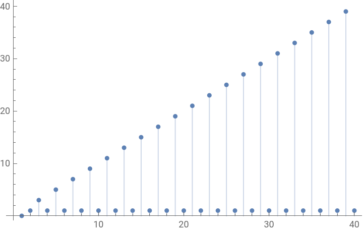
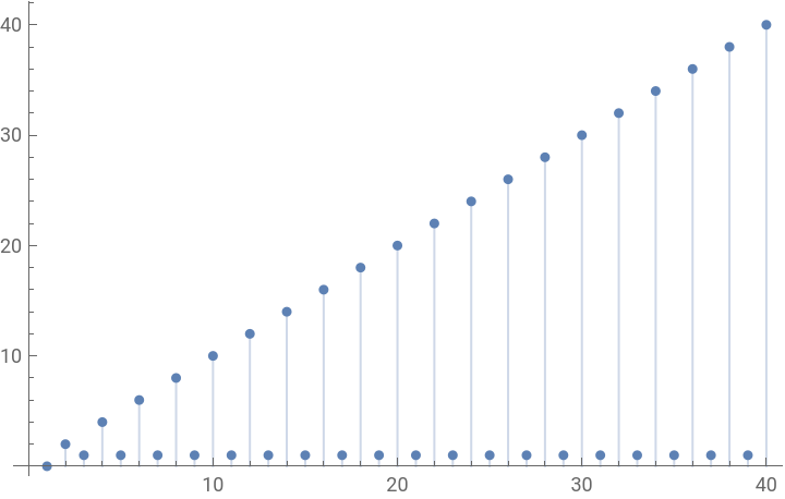
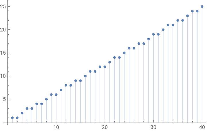
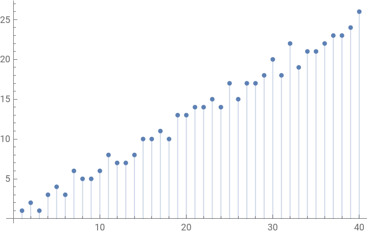
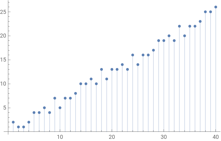
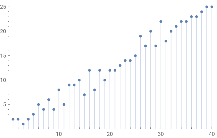
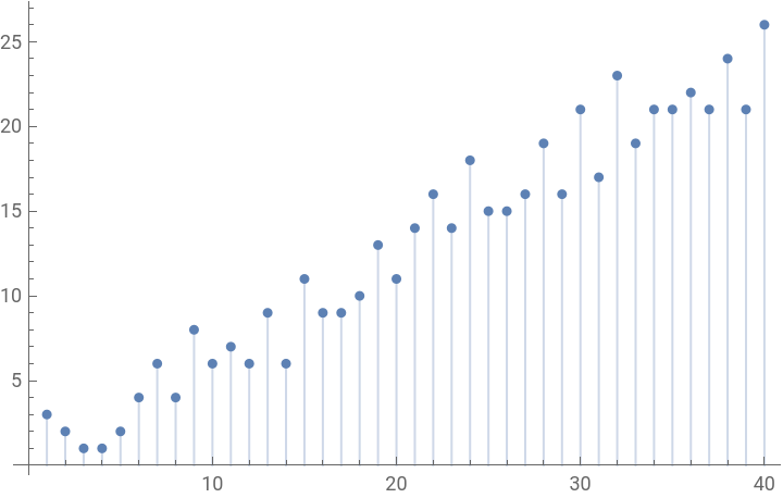
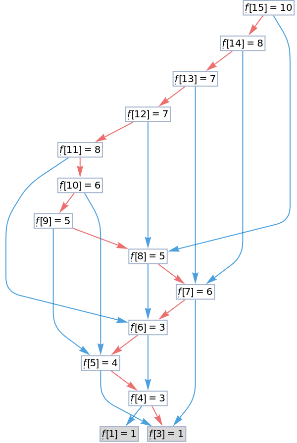
Careful examination shows that we’ve again rediscovered Hofstadter’s G-Function in the third column of the first row, and the blog’s headliner in the first item of the second row. Our alternative initial condition leads to the same call graph, other than two extra edges and an extra vertex:
Out[]=

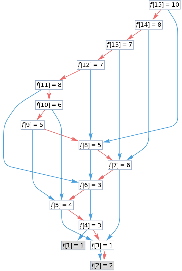
Of the five remaining items, three are non-trivial. Let’s first see what their call graphs look like in the manifold limit of many vertices:
Out[]=
|
|
|
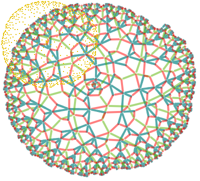
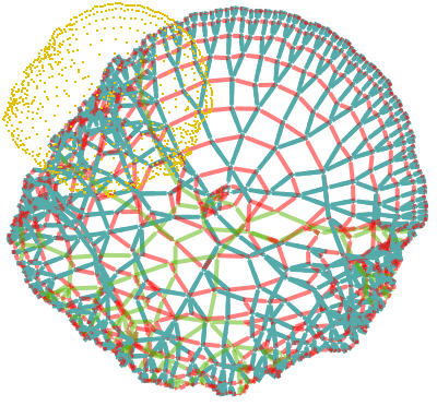
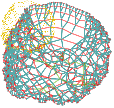
Wow! It already looks like we’re on to something cool here. Especially in the second and third graphs, we see emergence of order from chaos, where a radial subspace appears to contain a copy of the Hofstadter G-function’s Fibonacci-inspired call tree. Around the concentric spiral, we again see the triangle square pattern from “neat examples” of WFR`RecursiveFunctionCallGraph’s manual page:
Out[]=
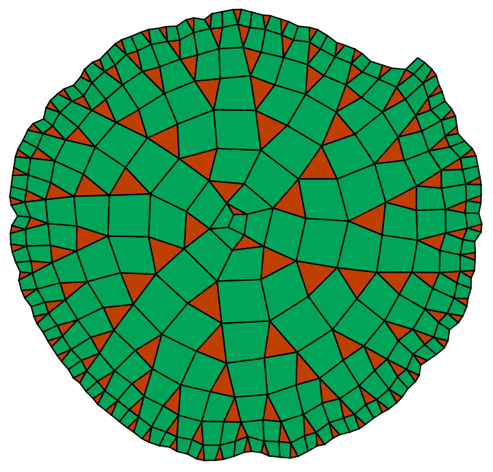
If we try to map the same depiction function over these messy graphs, we’re guaranteed to get some junk out, but not without bringing apparent similarities more sharply into focus:
Out[]=
|
|
|
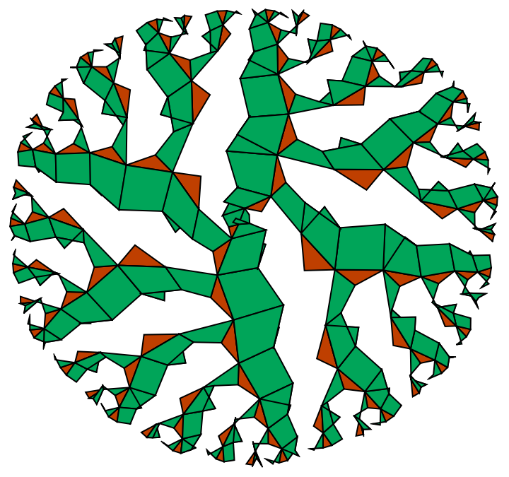
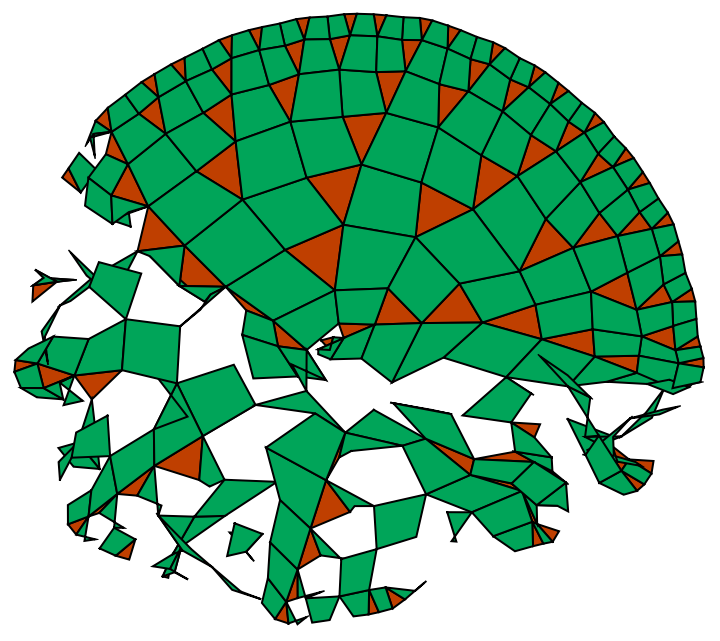
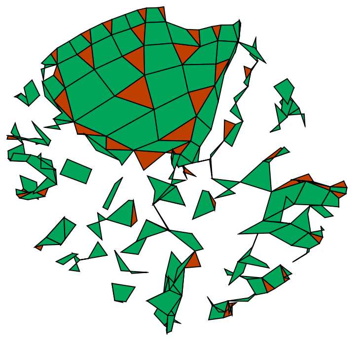
Even with this code mostly failing, we can see that the first item must have some sort of order to it. Let’s look more closely at it’s tree decomposition:
The left tree is strange, but it’s highly likely that a closed form for it will exist. The right tree almost obviously appears to be the “Fibonacci tree” discussed many places elsewhere. We can quickly test one instance:
and leave the proof for later. When the call graphs mix order and chaos, we can expect to see something similar using ListPlot on the function values themselves. Let’s subtract out the linear part, and take a look at what happens in the long run:
Again in the last two plots we see tight order interspersed with pseudo-randomness. Now let’s actually test the central dogma of chaos theory, which says that small changes in initial conditions lead to potentially large changes in the output value:
Up to length 15, we find a few missing words only for the first sequence, which is no surprise. Let’s take a look at the first sequence, by simply counting words of length four:
One of them is very rare, and we could guess, must occur near the initial conditions. If we chop the first term and look for omissions, we now find two rather than one:
This result suggests that we never find two consecutive evens flanked by odds, nor will we ever find two consecutive odds flanked by evens (other than one anomalous case around the initial values).
We can apply the same test to the difference of the two mostly-random sequences:
No surprise, we’re still finding all possible words. Just for the fun of it, let’s also look at the noise spectrum of the simple correlation function:
It seems not to have any significant pattern in the frequency domain, and if we listen to audio via ListPlay, it does indeed sound like noise:
We’ve now introduced a small but sufficient tool set for searching function space, and our next task will be to look at the space of all functions obtained by allowing different shift parameters and initial conditions.
Choosing initial conditions
Choosing initial conditions
[ As we have seen earlier, all call graphs in this family have a set of unique blue subtrees, one tree associated to each initial condition. In the plots above we’ve given different colors to values according to how they belong to one subtree or another. ]
As we have seen before with the Hofstadter G sequence, allowing for negative initial conditions can merge apparently separate trees by burying the unique root deeper on the negative side of the number line. In this case we can reduce from four to three initial conditions, and then the blue tree attains a common root:
Initially, our first colored ListPlot has four colors corresponding to the four unique subtrees (with blue edges). When allowing negative values, we’ve reduced to one subtree, so we could redraw the ListPlot using only one color. That isn’t necessary now, but it would be cool to find an algorithm that automatically reduces tree count by backing initial conditions to zero and negative inputs if possible. Anyone?
Let’s look closer at the one tree we’ve obtained. It does not quite have the Fibonacci branching from earlier, but it’s certainly doing something similar. If we simply count vertices on each level of the tree and divide by two, we already get back to the Fibonacci numbers:
Should we be surprised? Probably not, but if we really want to appreciate a fact, more work remains to be done proving why this pattern should continue to infinity. However, just now we are trying to get back quickly to the search for order.
Without having time for detailed analysis and bounding proofs, let’s just generate as many seemingly valid initial conditions as we possibly can:
With only 93 alternatives, analysis should be manageable. For each item input to WFR`RecursiveFunction, we will generate long sequences of over one million consecutive function values, and then submit the raw data to another function which reduces it mod 2, and subsequently identifies all missing binary words:
Next we do some post-processing and Sort by Max number of missing elements, and voila, one particular function stands out at the top of the set:
Before rushing on to see if the set of 256 missing words has any structure to it, we should search the next level to see if anything similar exists. The problem is that the next level already has thousands of elements:
The search can be expected to take significantly longer:
Leaving it on over night if necessary, we do obtain a few more similar results:
Even though we’re in a hurry and generating less data, this search still takes some time to complete:
Nothing immediately jumps out of the sorted results:
Which means that, for now, we can content ourselves with these few instances:
Next we will find out what these counts are really hiding.
Missing Gems
Missing Gems
In our exposition of the “hidden gems” sequences, let us first investigate how closely they conform to the hypothesis of Gaussian noise around a linearly increasing mean. When plotting values, most of what we see is apparent randomness:
However, the second and third items on the first row do look suspicious. Recurrent peaks of increasing magnitude are seen prominently here, and this systematic effect shows up again in histograms of function values around the linear expectation:
Other than artificially extended tails on the two items we mentioned previously, these graphs look like about what we would expect for Gaussian noise. Looks can be deceiving. Unlike our previous example from the introduction, we do not find a uniform Fourier spectrum. Instead we find pronounced peaks in each case:
This is a good second hint that something structural might be happening underneath all of the chaotic randomness in the generated data. What other randomness tests might these sequences fail?
We already know that all of these sequences have failed to generate all possible mixtures of even and odd terms. Now we can dive into the details by extracting the missing words and relating them through NearestNeighborGraph:
We’ve now searched thousands of functions, finding the “Missing Gems” phenomena at a prevalence of less than one percent. Many other functions have missing words, but those omissions are typically not localized to one word length, nor do the associated adjacency graphs have the symmetrical feature of vertex transitivity. What we’re looking at seems to be rare, and difficult to explain. Can we find more examples? Can anyone actually **prove** why these sequences should have hypercube-shaped omissions (or not)?
The “Missing Gems” Sequence
The “Missing Gems” Sequence
Not only is this the simplest known example in terms of parameter counting, it also is the most simple in terms of tree count. It’s call-back graph has only two trees, one persistent and the other transient:
Too bad, we’re stuck with one transient tree and an extra initial condition. Oh well, moving on, let’s look in more detail at the persistent tree:
Again on the left side, we see terminal leaves due to skipped values. Meanwhile, the branching at each vertex is much more unpredictable than for the previous Fibonacci tree. Counting vertices per level we get:
The branching ratios seem to settle down to about GoldenRatio:
It’s not clear if the maximum branching reaches a plateau or grows unboundedly:
The first few terms of the parity sequence are:
Per what we’ve already discovered, we know that interesting behaviors of the parity sequence will be revealed when considering consecutive and overlapping subsequences of length 10. Let’s immediately define a few more derived sequences:
The missing gems non-membership sequence visits most integers in the range [0,15], but not those associated with the hidden gems:
What we’re really getting at here is the shift structure of the parity sequence. Now let’s consider the encoding of ten-digit binary words to integers, and define another important sequence.
This sequence is expected to visit most integers in [0, 1023], but as we’ve seen already, it is also expected to miss exactly 256 values:
Just to re-iterate, the missing gems conjecture states that--after transforming the missing gems sequence to binary, parting out words of length ten, and then encoding them to integers--that the encodings sequence never visits the following 256 missing words:
If the Missing Gems conjecture is true, these 256 vertices will ultimately drop out of the DeBruijin graph, leading to a state transition graph with more unusual structure. The general DeBruijin graph is here:
Deleting vertices associated with Missing Gems, we get something slightly different:
Since the unique determination property applies just as well to left shift as it does to right shift, we find at each vertex that the out degree equals the in degree:
Why should this fact matter at all? There are 384 / 1024 words with a unique successor and unique predecessor:
These special words can also be extracted directly from the reduce DeBruijin graph:
These 384 alternatives give us another way to calculate the determined shift sequence (as defined above), and here are the first few terms again:
It’s also worth mentioning another sequence, which divides edges of the reduced DeBruijin graph into four classes.
Using this sequence, we can color the edges of the DeBruijin graph:
We’ve already made quite a mess without proving much of anything, but how can we stop now, when we haven’t even looked into the structure of the reduced DeBruijin graph? If we only look at the subgraph which allows appending either a 0 or a 1, we get ten components, nine of which are isomorphic cycles with attached rhombi allowing for input and output:
The check for missing words in the out component passes easily:
Next we re-attach “dangerous” vertices, where--if the missing Gems conjecture is false--it could be possible to turn off toward a missing word:
These ten components have considerable overlap:
An interesting question is whether or not any pair of cycle graphs combine into a prism. Certainly not the first and fourth item, which are the only way to access the tenth, as seen here:
If we group by cycle count, most of the prism subgraphs occur in the set with only four unique cycles:
Wow, even more order produced from chaos, how beautiful! Unfortunately, it seems like we’re still quite a ways away from proving the Missing Gems conjecture, but perhaps someday we’ll figure it out.
Broader Context
Broader Context
We’ve limited ourselves to a narrow scope by choosing a particular functional form. In principle, we can apply the binary words randomness test to any integer sequence, and might again find missing words with interesting adjacency structure. Then again, maybe not. Let’s just sample a few items from the OEIS, run the test, and see what we get.
But the counts are low enough to preclude any interesting adjacency structure as seen before. Indeed we’ve looked closer at the sets, finding no remarkable symmetry. Meanwhile, the Hofstadter Q Function doesn’t have any missing binary words, at least up to length 15:
Similarly, we searched OEIS entries A055748, A070867, and A070868 finding nothing. We then searched A006949 finding a few missing words but no interesting structures between them. There’s no reason to expect missing words from a pseudo-random number generator, and indeed A096550 didn’t show any. Another plausible place to look would be permutations of the natural numbers. Two that I remember from previously are A064413 and A098550. Their counts sequences did have some non-zero values, but again nothing as unusual as what we’ve already seen with the missing gems.
We would really like to do more searching of known results, but don’t know exactly where to look in OEIS’s thousands and thousands of examples. If we search middle columns of elementary Cellular Automata, such as A051023 for rule 30, then we find 30, 45, 75, 86, 89, 101, 135, 149 at least generate every binary word up to length 10, while other central columns encounter missing words fairly quickly. Again, no more missing gems.
This is another important question that might inspire someone to do some basic analysis on OEIS entries: Can we find any other integer sequence, which is random enough to generate most words (say up to length 5 or 6), then eventually finds an isolated set of missing words with some sort of intrinsic symmetry?
Conclusion
Conclusion
In this present effort, we’ve looked at relatives of Hofstadter’s G sequence, finding some interest in functions which generate imperfect randomness. Another chapter from Hofstadter’s “Godel Escher Bach” comes to mind as immediately relevant in the contextualization of our results: The MU puzzle, which can also be read as an allusion to the first case of “The Gateless Gate”(mu = 無, in Japanese). In the MU puzzle, the reader is asked to transform a word “MI” to another word “MU” by using a certain set of re-write rules. The point of the puzzle is that the solution is not possible, because the set of all possible words divides into reproducible and non-reproducible, and MU is provably non-reproducible (or in atavistic Chinese, some words are 無, while others are 有, but MU is definitely 無).
Our version of the “MU” puzzle is slightly more complicated. Using relatively difficult production rules, we’ve found many missing words (無詞), which arrange nicely into missing gems (無珠). Not only that, but in our exploration of DeBruijin graphs, we’ve found even more prismatic gems in the positive space (有珠). Don’t get me wrong--we’re not claiming to have found the Cintamani mentioned in the Ocean Seal Diagram! Trying to mythologize mathematics is a very bad idea akin to gilding the lily, or gilding the lotus if you’d rather. On the other hand, trying to mathematicize mythology can be an effective strategy. Our mathematical study of missing gems does nothing to make fantastical mythological treasure hunting more natural. Yet, from a pure maths point of view, the idea of gems appearing out of formless chaos now seems less bizarrely imaginative.
In any case, we’re not here just to formulate a dignified opinion whether Chaos (混沌) is more like Presence (有) or Absence (無). We’ve just now observed that the missing gems (無珠) exist for millions of terms and have only conjectured that they will persist to infinity. Can anyone prove the missing gems conjecture? And while we’re waiting for an answer on that one, can anyone find other distinct examples of the missing gems phenomena? It seems much work remains to be done on this front...
Acknowledgements
Acknowledgements
Thanks to Stephen Wolfram for breaking assumptions about initial conditions. This lead to the discovery of the second distinct missing gems sequence. Thanks to Thomas Adler for contributing to the WFR code.
CITE THIS NOTEBOOK
CITE THIS NOTEBOOK
Finding missing gems amidst chaos
by Brad Klee
Wolfram Community, STAFF PICKS, October 3, 2024
https://community.wolfram.com/groups/-/m/t/3289552
by Brad Klee
Wolfram Community, STAFF PICKS, October 3, 2024
https://community.wolfram.com/groups/-/m/t/3289552