Nestedly Recursive Functions extend traditional recursion by embedding self-referential calls within layered structures, leading to complex and often unpredictable computational behaviors. This project studies a specific Nestedly Recursive Function which could simulate 2-tag system, that is Turing complete. This shows NRF is indeed capable of universal computation, and sheds light into a deeper question: “what is the simplest universal nested recursive function?”.
1:Project Background
1:Project Background
1.1:Introduction to Nestedly Recursive Functions
1.1:Introduction to Nestedly Recursive Functions
Nestedly Recursive Functions (NRF) are essentially functions that, when evaluated, access recursively other values on their domain. An example is:
F(n)n-F(F(n-1)),F(1)F(3)1
NRF leads to complex and often unpredictable computational behaviors. As explored by Stephen Wolfram in Nestedly Recursive Functions, these functions arise in combinatorics, formal systems, and foundational computation, revealing deep connections between recursion and universality.
A nested recurrence relation is said to be undecidable if the following problem is undecidable: given a finite set of initial conditions for , is the recurrence relation calculable? Here calculable means that for every , either is an initial condition or the calculation of involves only invocations of on arguments in .
A(n)
A(n)
n≥0
A(n)
A(n)
A
{0,1,...,n-1}
1.2:Introduction to 2-tag system
1.2:Introduction to 2-tag system
A 2-tag system is a computationally universal string rewriting model with a finite alphabet that operates by iteratively deleting a fixed number of leading 2 symbols and appending new symbols based on simple production rules. Despite their minimalistic design, these systems can simulate Turing machines and exhibit complex computational behaviors.
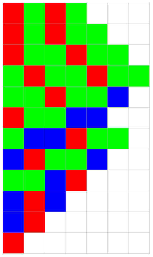
A 2-tag systems is depicted below, which uses alphabet , an initial string abab and production rules given by:
Σ{a,b,c}
W
0
Δ
Δ:aabb,bc,ca
In[]:=
TagSystemNew[2,{"a"->"abb","b"->"c","c"->"a"},Characters@"abab"]
Out[]=
{abab,ababb,abbabb,babbabb,bbabbc,abbcc,bccabb,cabbc,bbca,cac,ca,a}
We use red to represent , and green for , blue for , and produce an array plot.
a
b
c
In[]:=
TagPlot@TagToIntList@TagSystemNew[2,{"a"->"abb","b"->"c","c"->"a"},Characters@"abab",20]//Grid[{{#},{"2-Tag System"}},Frame->All]&
Out[]=
2-Tag System |
2:Simulating 2-tag system with a NRF
2:Simulating 2-tag system with a NRF
The question being attacked here “can a nestedly recursive function be universally computable”, or more specifically in this scenario, “is there such a NRF that is capable of simulating any 2-tag system?”
The formulation studied and presented here was proposed by An Undecidable Nested Recurrence Relation. Such construction relies on tag system writing one symbol at a time, what leads to another computational model.
The formulation studied and presented here was proposed by An Undecidable Nested Recurrence Relation. Such construction relies on tag system writing one symbol at a time, what leads to another computational model.
2.1:Reverse tag system
2.1:Reverse tag system
A reverse tag system consists of a finite set of symbols , a set of production rules , a function , and an initial word ∈. While an ordinary tag system modifies a word by removing a fixed number of symbols from the beginning and adding a variable number of symbols to the end, the situation is reversed in a reverse tag system. A single computation step of a reverse tag system is described by the operation
Σ
δ:Σ
2
Σ
d:ΣN
W
0
*
Σ
w
1
w
k
w
d(y)+1
w
k
where . Given a word that starts with and ends with , the production rule for the pair yields a symbol which is appended to the end of the word. Then, the first symbols are removed from the beginning of the word. If at some point the exceeds k, then the reverse tag system halts.
yσ(,)
w
1
w
k
w
1
w
k
(,)
w
1
w
k
y
d(y)
d(y)
2.2:Reverse tag system to 2-tag system
2.2:Reverse tag system to 2-tag system
We follow by showing how one can use reverse tag system to simulate/run 2-tag system.Consider a 2-tag system , let be the maximum length of strings replaced in the substitution rules, and be an alphabet of size u times the length of , where each letter consists of an original letter from augmented with subscripts .For each ∈Σ, write as ....The production rules of include the rules
T(Σ,Δ,)
W
0
u
′
Σ
Σ
Σ
u
1,2,...,u
s
i
Δ()
s
i
s
i,
l
i
s
i,2
s
i,1
δ
δ(,)
[]
s
i
*
[*]
1
[]
s
i,
l
i
l
i
δ,
[]
s
i
*
[]
s
i,j
j
[]
s
i,j-1
j-1
where represents an arbitrary symbol or subscript.
*
The deletion numbers are specified by
d
[s]
j
0 | if j>1 |
2 | if j1 |
Finally let be the result of adding a superscript to each character in .
′
W
0
1
W
0
Now we say reverse tag system simulates 2-tag system . It can be proven that extracting every step where delete function gives from (ignoring the subscripts) yields the execution steps of .
R(,δ,d,)
′
Σ
′
W
0
T(Σ,Δ,)
W
0
2
R
T
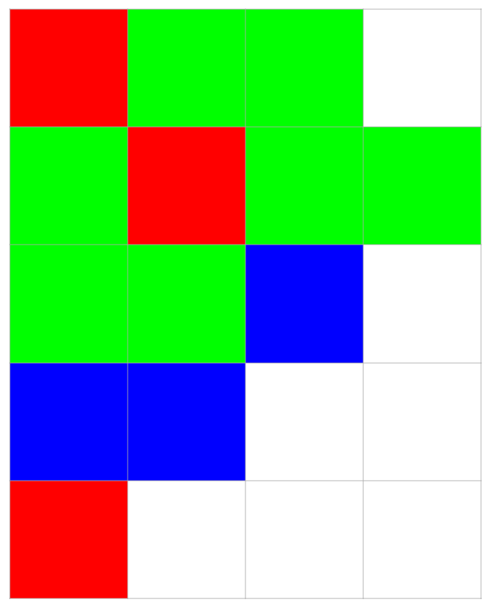
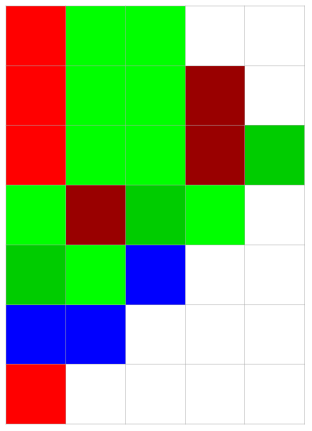
See some examples of tag systems X their reverse tag system version being simulated:
In[]:=
With[{rule={"a"->"abb","b"->"c","c"->"a"},initial=Characters@"abb"},{revSymbols,revInitials,revRulesA,revRules,RevDelete}=TagToReverseTagSystem[2,rule,initial];{TagPlot@TagToIntList@TagSystemNew[2,rule,initial,20],TagPlot@RevTagToIntList@ReverseTagSystem[revRules,RevDelete,revInitials,20]}]//Grid[{#,{"2-Tag","Reverse 2-Tag"}},Frame->All]&
Out[]=
2-Tag | Reverse 2-Tag |
2.3: Reverse tag system to B(n)
2.3: Reverse tag system to
B(n)
We define a conditional NRF (defined on natural numbers) as
B(n)
B(n)
B(n-2)+2B(B(n-1)) | if n is even, |
B(2B(n-2-B(n-1))+B(n-2)) | if n is odd. |
And we aim to simulate a reverse tag system by carefully selecting the initial condition of - in fact this is the only way one can encapsulate information in a potential computational NRF.
R(Σ,δ,d,)
W
0
B(n)
Assuming , a function is defined as follows:
Σ{,,...,}
s
1
s
2
s
t
α
α()+2+2
s
i
i+1
4
2i+2
2
α(,)2α()+α()++6
s
i
s
j
s
i
s
j
2i+3
2
2j+2
2
The fact that is injective can be seen by considering the binary representation of such numbers.
The encoding for and is done respectively as follows:
α
The encoding for
d
δ
B(α())1-d()
s
i
s
i
B(α(,))αδ(,)
s
i
s
j
s
i
s
j
Let α(,)+2, we encode (suppose ...) as follows:
c
0
s
t
s
t
W
0
W
0
q
1
q
2
q
m
B(+2k-1)α(),1≤k≤m
c
0
q
k
Specifically, we let , and let if and hasn’t been defined above.
B(+2m)2m-2
c
0
B(k)0
0≤k<+2m
c
0
B(k)
Suppose that at the th computation step of , the word is produced. It can be proven that the following equalities hold :
i
R
W...
w
1
w
2
w
k
(B(n-2k+1),...,B(n-3),B(n-1))(α(),α(),...,α())
w
1
w
2
w
k
B(n)2k-2
where .
n+2m+2i
c
0
Thus we can say with the initial condition given above simulates .
But the function itself is conditional, so we still need one extra step in order to provide a “truly” Nested Recursive Function:.
B(n)
R(Σ,δ,d,)
W
0
But the function itself is conditional, so we still need one extra step in order to provide a “truly” Nested Recursive Function:
A(n)
In[]:=
With[{rule={"a"->"abb","b"->"c","c"->"a"},initial=Characters@"abb"},{revSymbols,revInitials,revRulesA,revRules,RevDelete}=TagToReverseTagSystem[2,rule,initial];{BG,steps}=ReverseTagToBGraph[revSymbols,revInitials,revRulesA,revRules,RevDelete];BG[steps-1]]
Out[]=
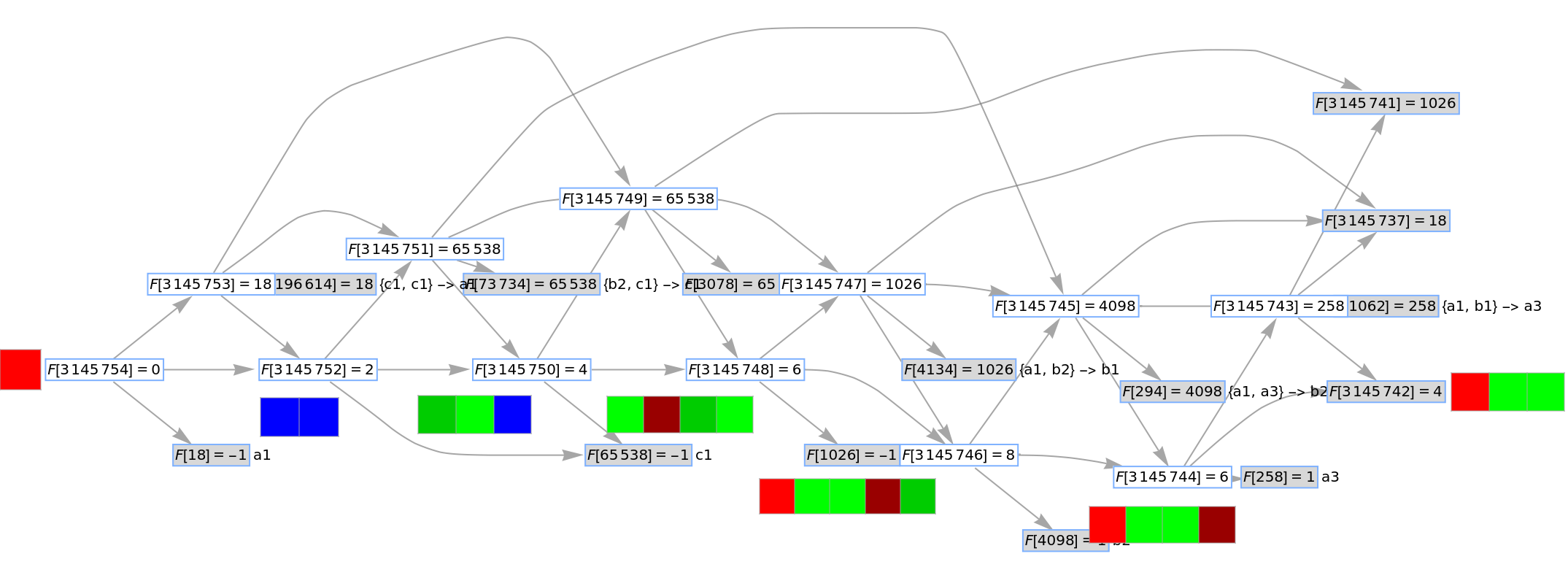
The following gif show how computes step by step:
B(n)
In[]:=
With[{rule={"a"->"abb","b"->"c","c"->"a"},initial=Characters@"abb"},{revSymbols,revInitials,revRulesA,revRules,RevDelete}=TagToReverseTagSystem[2,rule,initial];{BG,steps}=ReverseTagToBGraph[revSymbols,revInitials,revRulesA,revRules,RevDelete];graphList=BG/@Range[0,steps-1];coordinates=Thread[VertexList[Last@graphList]->GraphEmbedding[Last@graphList]];Graph[#,ImageSize->1400,PlotRange->{{-5.5,9.5},{0.5,5.5}},GraphLayout->{"LayeredDigraphEmbedding","Orientation"->Left},VertexCoordinates->coordinates,EdgeShapeFunction->"CurvedArc",EdgeStyle->Arrowheads[0.05]]&/@graphList]//ListAnimate
Concluding Remarks
Concluding Remarks
Acknowledgments
Acknowledgments
Pietro Pepe, Stephen Wolfram
References
References
1
.Stephen Wolfram (2024), “Nestedly Recursive Function,”.https://writings.stephenwolfram.com/2024/09/nestedly-recursive-functions/
2
.A. Marcel Celaya and B. Frank Ruskey (2012), “An Undecidable Nested Recurrence Relation”. https://arxiv.org/pdf/1203.0586
Cite This Notebook
Cite This Notebook
“Computability on Nestedly Recursive Functions (NRF)”
by Bowei Xv
Wolfram Community, 2025.7.9
https://community.wolfram.com/groups/-/m/t/3497880
by Bowei Xv
Wolfram Community, 2025.7.9
https://community.wolfram.com/groups/-/m/t/3497880