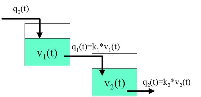
Assume volumetric flow rate proportional to liquid volume in the tank : (t)=(t) where i=1, 2. Initially the two tanks are empty.
q
i
k
i
v
i
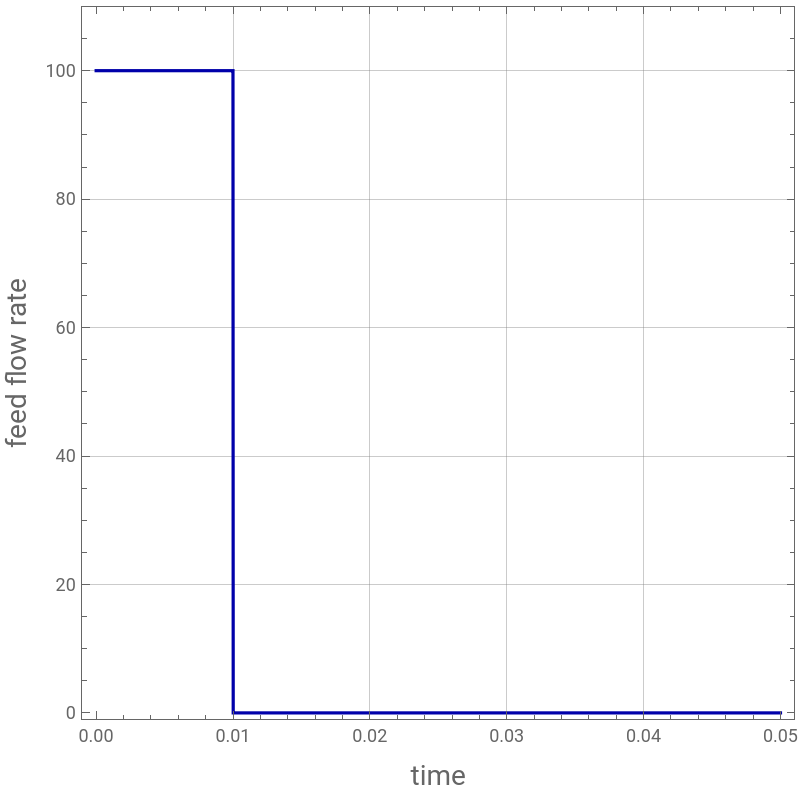
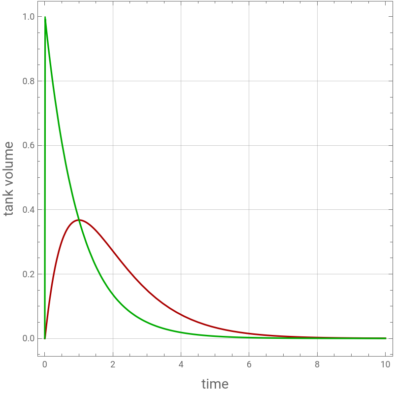
Dynamic response to a pulse in feed flow rate
In[]:=
q[t_]:=ϵ (UnitStep[t]-UnitStep[t-1/ϵ])
In[]:=
ϵ=100;
In[]:=
Plot[q[t],{t,0,5/ϵ},PlotStyleDarker@Blue,AspectRatio1,GridLinesAutomatic,
FrameTrue,ImageSize400{1,1},PlotRange{-1,110},FrameLabel{Style["time",14],Style["feed flow rate",14]}]
FrameTrue,ImageSize400{1,1},PlotRange{-1,110},FrameLabel{Style["time",14],Style["feed flow rate",14]}]
Out[]=
In[]:=
sol1=NDSolve[{(D[[t],{t,1}]q[t]-k[t])/.k1,(D[[t],{t,1}]k[t]-k[t])/.k1,[0]0,[0]0},{[t],[t]},{t,0,100}]
v
1
v
1
v
2
v
1
v
2
v
1
v
2
v
1
v
2
Out[]=
[t]InterpolatingFunction[t],[t]InterpolatingFunction[t]
v
1


v
2

In[]:=
plt1=Plot[{[t]/.sol1,[t]/.sol1},{t,0,10},PlotStyle{Darker@Red,Darker@Green},AspectRatio1,GridLinesAutomatic,FrameTrue,ImageSize400{1,1},PlotRangeAll,FrameLabel{Style["time",14],Style["tank volume",14]},PlotLegends{Style["tank 1",14],Style["tank 2",14]},PlotRangeAll]
v
2
v
1
Out[]=


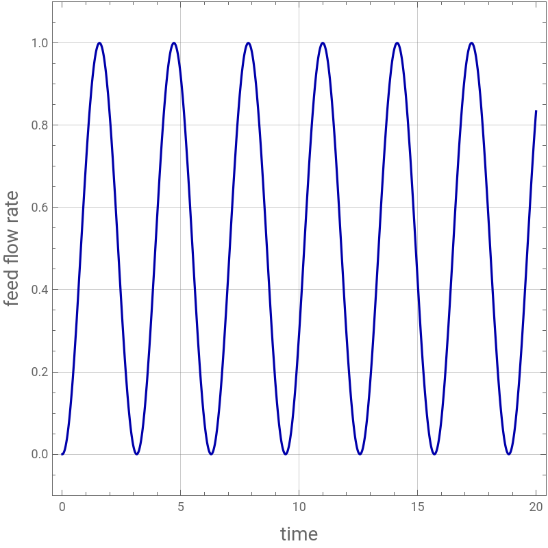
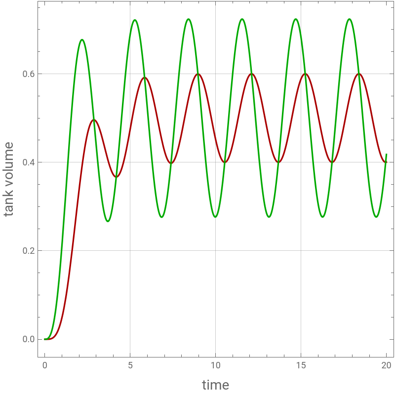
Dynamic response to a specific feed flow rate (for example a wave)
2
Sin
In[]:=
q[t_]:=Sin[t]^2
In[]:=
plt2=Plot[q[t],{t,0,20},PlotStyleDarker@Blue,AspectRatio1,GridLinesAutomatic,
FrameTrue,ImageSize400{1,1},PlotRange{-0.1,1.1},FrameLabel{Style["time",14],Style["feed flow rate",14]}]
FrameTrue,ImageSize400{1,1},PlotRange{-0.1,1.1},FrameLabel{Style["time",14],Style["feed flow rate",14]}]
Out[]=
In[]:=
sol2=NDSolve[{(D[[t],{t,1}]q[t]-k[t])/.k1,(D[[t],{t,1}]k[t]-k[t])/.k1,[0]0,[0]0},{[t],[t]},{t,0,100}]
v
1
v
1
v
2
v
1
v
2
v
1
v
2
v
1
v
2
Out[]=
[t]InterpolatingFunction[t],[t]InterpolatingFunction[t]
v
1

v
2

In[]:=
plt3=Plot[{[t]/.sol2,[t]/.sol2},{t,0,20},PlotStyle{Darker@Red,Darker@Green},AspectRatio1,GridLinesAutomatic,FrameTrue,ImageSize400{1,1},PlotRangeAll,FrameLabel{Style["time",14],Style["tank volume",14]},PlotLegends{Style["tank 1",14],Style["tank 2",14]},PlotRangeAll]
v
2
v
1
Out[]=
Obtaining the same dynamic response using the convolution theorem and the impulse response (i.e., sol1 found above).
The solution obtained using the convolution theorem is represented with gray dots.
The solution obtained using the convolution theorem is represented with gray dots.
In[]:=
Off[NIntegrate::slwcon]
In[]:=
Off[NIntegrate::ncvb]
Problem is suitable for parallel calculations using LaunchKernels and Parallelize
In[]:=
LaunchKernels[]
Out[]=
KernelObject,KernelObject,KernelObject,KernelObject
In[]:=
f[τ_]:=NIntegrate[First[[t]/.sol1]q[τ-t],{t,0,τ}]
v
1
In[]:=
tblv1=Parallelize@Table[{x,f[x]},{x,0.1,20,0.1}]
Out[]=
{{0.1,0.000279374},{0.2,0.00233899},{0.3,0.00782309},{0.4,0.0180752},{0.5,0.0341001},{0.6,0.056538},{0.7,0.0856515},{0.8,0.121327},{0.9,0.16309},{1.,0.210133},{1.1,0.261356},{1.2,0.315419},{1.3,0.370801},{1.4,0.42587},{1.5,0.47895},{1.6,0.528395},{1.7,0.57266},{1.8,0.610366},{1.9,0.640357},{2.,0.661754},{2.1,0.673989},{2.2,0.676832},{2.3,0.670404},{2.4,0.655172},{2.5,0.631935},{2.6,0.601792},{2.7,0.566102},{2.8,0.52643},{2.9,0.484484},{3.,0.442054},{3.1,0.400935},{3.2,0.362863},{3.3,0.32944},{3.4,0.302078},{3.5,0.281937},{3.6,0.269885},{3.7,0.266458},{3.8,0.271846},{3.9,0.285881},{4.,0.308047},{4.1,0.337498},{4.2,0.373096},{4.3,0.413451},{4.4,0.456986},{4.5,0.501988},{4.6,0.546689},{4.7,0.589327},{4.8,0.628222},{4.9,0.661839},{5.,0.688856},{5.1,0.708208},{5.2,0.719137},{5.3,0.721219},{5.4,0.714382},{5.5,0.698908},{5.6,0.675422},{5.7,0.644868},{5.8,0.608472},{5.9,0.56769},{6.,0.524155},{6.1,0.479608},{6.2,0.435828},{6.3,0.394566},{6.4,0.35747},{6.5,0.326024},{6.6,0.301483},{6.7,0.284829},{6.8,0.276729},{6.9,0.277507},{7.,0.287135},{7.1,0.305231},{7.2,0.331076},{7.3,0.36364},{7.4,0.401627},{7.5,0.443523},{7.6,0.48766},{7.7,0.532278},{7.8,0.575601},{7.9,0.615902},{8.,0.651574},{8.1,0.681197},{8.2,0.70359},{8.3,0.717861},{8.4,0.723442},{8.5,0.72011},{8.6,0.707999},{8.7,0.687593},{8.8,0.659704},{8.9,0.625445},{9.,0.586182},{9.1,0.543481},{9.2,0.499044},{9.3,0.454644},{9.4,0.41205},{9.5,0.37296},{9.6,0.338934},{9.7,0.311327},{9.8,0.291241},{9.9,0.279477},{10.,0.276503},{10.1,0.282438},{10.2,0.297046},{10.3,0.319744},{10.4,0.349628},{10.5,0.385506},{10.6,0.425948},{10.7,0.469342},{10.8,0.513958},{10.9,0.558016},{11.,0.599762},{11.1,0.63753},{11.2,0.669814},{11.3,0.695329},{11.4,0.713056},{11.5,0.722289},{11.6,0.72266},{11.7,0.714154},{11.8,0.69711},{11.9,0.672208},{12.,0.64044},{12.1,0.603073},{12.2,0.561597},{12.3,0.517665},{12.4,0.473029},{12.5,0.429468},{12.6,0.388719},{12.7,0.352406},{12.8,0.321977},{12.9,0.298645},{13.,0.283341},{13.1,0.276674},{13.2,0.278911},{13.3,0.289961},{13.4,0.309385},{13.5,0.336408},{13.6,0.369953},{13.7,0.408683},{13.8,0.451053},{13.9,0.495374},{14.,0.53988},{14.1,0.582796},{14.2,0.622411},{14.3,0.657146},{14.4,0.685616},{14.5,0.706686},{14.6,0.719516},{14.7,0.723595},{14.8,0.718759},{14.9,0.705203},{15.,0.683465},{15.1,0.654414},{15.2,0.619206},{15.3,0.579246},{15.4,0.536127},{15.5,0.491567},{15.6,0.447344},{15.7,0.40522},{15.8,0.366874},{15.9,0.333836},{16.,0.307422},{16.1,0.288686},{16.2,0.278374},{16.3,0.276897},{16.4,0.284315},{16.5,0.300332},{16.6,0.324309},{16.7,0.35529},{16.8,0.39204},{16.9,0.433094},{17.,0.476816},{17.1,0.521461},{17.2,0.565252},{17.3,0.60644},{17.4,0.643386},{17.5,0.674615},{17.6,0.698882},{17.7,0.715221},{17.8,0.72298},{17.9,0.721849},{18.,0.711874},{18.1,0.693452},{18.2,0.667317},{18.3,0.634513},{18.4,0.596345},{18.5,0.554337},{18.6,0.510162},{18.7,0.465583},{18.8,0.422375},{18.9,0.382262},{19.,0.346843},{19.1,0.31753},{19.2,0.295491},{19.3,0.281605},{19.4,0.276426},{19.5,0.280161},{19.6,0.292659},{19.7,0.313424},{19.8,0.341627},{19.9,0.376143},{20.,0.415598}}
In[]:=
plt4=ListPlot[tblv1,PlotStyle{Darker@Gray,PointSiez[0.015]}];
In[]:=
plt2=Plot[q[t],{t,0,20},PlotStyleDarker@Blue,AspectRatio1,GridLinesAutomatic,
FrameTrue,ImageSize400{1,1},PlotRange{-0.1,1.1},FrameLabel{Style["time",14],Style["",14]}];
FrameTrue,ImageSize400{1,1},PlotRange{-0.1,1.1},FrameLabel{Style["time",14],Style["",14]}];
In[]:=
Show[plt2,plt3,plt5,plt4]
CITE THIS NOTEBOOK
CITE THIS NOTEBOOK
Impulse response of two tanks in series
by Housam Binous and Ahmed Bellagi
Wolfram Community, STAFF PICKS, July 21, 2023
https://community.wolfram.com/groups/-/m/t/2974203
by Housam Binous and Ahmed Bellagi
Wolfram Community, STAFF PICKS, July 21, 2023
https://community.wolfram.com/groups/-/m/t/2974203