This notebook series is designed to introduce selected dynamic economic models to both advanced undergraduate and graduate students. Economists have relied on a series of economic models to better understand the otherwise highly complex causal relationship among many economic variables. Dynamic economic models set up by systems of either difference or differential equations are particularly useful in tracing the change in the quantity of unknown economic variables (e.g., the capital stock, demand for labor, aggregate output, etc.) and their interactions over time.
This notebook series aims to help students better understand the depth, usefulness, and limitations of major existing micro and macroeconomic models by demonstrating how we can use Wolfram Mathematica to replicate and reconstruct the core ideas and find dynamic solution of the model.
The model introduced in this notebook series include, among others, (1) the cobweb model of the quantity and price adjustment, (2) Keynes’s aggregate demand model, (3) Hicks’s ISLM model, (4) Samuelson’s investment accelerator model, (5) Kalecki’s investment delay model, (6) the predator-prey interaction model, (7) the epidemic model, (8) Ricardo’s three dimensional business cycle model, (9) Marx-Goodwin business cycle and growth model, (10) Smith’s and Ricardo’s growth model, (11) the Harrod-Domar growth model, (12) the Solow growth model, (13) the RBC model, (14) Romer’s new growth model, and (15) the circuit of capital model.
Introduction
Introduction
The Harrod-Domar model is one important growth model presented and discussed by Cambridge Keynesian economists in the late 1930s and 40s. The model begins with identifying the spending side of aggregate output-income and derives the equation for the growth rate of aggregate output-income as a function of three parameters that are crucial to this model. These are the savings rate, capital-output ratio, and the depreciation rate of the capital stock.
This note represents the core ideas of this model and its derivation procedure to trace the dynamic solution behavior. One important feature of this model is that the growth process is of the kind of the exponential growth pattern but with highly unstable fluctuations in the growth trajectory. This feature is a stark contrast with what Robert Solow predicted about 20 years later. The interested readers can consult Domar’s original paper (Domar 1946) and Chiang and Wainwright (2005)’s introduction to this model suggested in the reference section.
The model structure
The model structure
The spending side of aggregate output-income
The spending side of aggregate output-income
Domar begins with the following spending side of the national income (i.e., GDP):
Y=C+S=C+sY=C+I
(
1
)where Y is the aggregate output-income (or national income), C total consumption and S total savings, the latter of which is a certain fixed proportion of aggregate output-income, sY. At equilibrium, this aggregate saving is entirely used to finance the private business investment spending, I.
The derivation of the growth rate of aggregate output-income
The derivation of the growth rate of aggregate output-income
The growth of the capital stock can be denoted by the following difference equation:
K[t+1]=K[t]-δK[t]+sY[t]
(
2
)where δ represents the constant depreciation of the existing capital stock and sY[t] is the investment spending at time t.
If we introduce and define a new parameter v ≡ K/Y, the capital-output ratio, then K = vY holds true. This parameterized capital stock equation allows us to rewrite the previous capital stock equation into:
vY[t+1]=vY[t]-δvY[t]+sY[t]=(1-δ)vY[t]+sY[t]
(
3
)Subtracting vY[t] from both sides of the equation, we get
vY[t+1]-vY[t]=(1-δ-1)vY[t]+sY[t]
(
4
)Dividing through by vY[t], we arrive at
vY[t+1]-vY[t]
vY[t]
Y[t+1]-Y[t]
Y[t]
sY[t]
vY[t]
s
v
(
5
)The left-side of the equation is the growth rate of national income, which is equated with the ratio of the three parameters, s/v - δ. If we assume that the depreciation of the existing capital stock is negligible, the growth rate of national income is determined by the savings rate and the capital-output ratio.
The solution to the system of difference equations
The solution to the system of difference equations
A system of the two first-order difference equations
A system of the two first-order difference equations
Alternatively, from (2) and (3) we can derive the following system of two difference equations, one for the capital stock and the other for aggregate output-income:
K[t+1]=K[t]-δK[t]+sY[t]Y[t+1]=(1-δ)Y[t]+(s/v)Y[t]
(
6
)The analytical solution
The analytical solution
The general solution to this system of difference equations, assuming that the initial value of K[0] and Y[0] are given by K0 and Y0 respectively, can be found by:
In[]:=
Clear[s,v,δ,Y,Y0,K,K0,t,sol1];RSolve[{K[t+1]==(1-δ)K[t]+sY[t],Y[t+1]==(1-δ)Y[t]+(s/v)Y[t],K[0]==K0,Y[0]==Y0},{Y[t],K[t]},t]
Out[]=
K[t]K0-vY0+vY0,Y[t]Y0
t
(1-δ)
t
(1-δ)
t
1+-δ
s
v
t
s+v-vδ
v
Out[]=
K[t]K0-vY0+vY0,Y[t]Y0
t
(1-δ)
t
(1-δ)
t
1+-δ
s
v
t
s+v-vδ
v
A static visualization of the solution curve with fixed parameters
A static visualization of the solution curve with fixed parameters
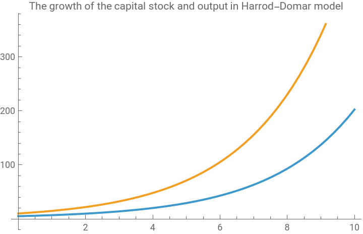
Suppose we have the following parameters and the two initial conditions. Then the solution curve will be:
In[]:=
Clear[s,v,δ,Y,Y0,K,K0,t,sol1];s=0.2;δ=0.02;v=0.4;K0=5;Y0=10;sol1=RSolve[{K[t+1]==(1-δ)K[t]+sY[t],Y[t+1]==(1-δ)Y[t]+(s/v)Y[t],K[0]==K0,Y[0]==Y0},{K[t],Y[t]},t]Plot[Evaluate[{K[t],Y[t]}/.sol1],{t,0,10},PlotLabel->"The growth of the capital stock and output in Harrod-Domar model",PlotLegends->{"K(t)","Y(t)"}]
Out[]=
{{K[t]-4.(-1.25+1.-1.),Y[t]10.}}
-1.t
1.02041
t
0.98
1.t
1.02041
1.t
1.02041
t
1.48
t
1.48
Out[]=


The solution to the system of differential equations
The solution to the system of differential equations
A system of the two first-order differential equations
A system of the two first-order differential equations
In a differential equation form, we can rewrite the growth rate of aggregate output-income in the following way:
Y
Y(t)
s
v
(
7
)This is the same thing as:
Y
s
v
(
8
)Combining this with a differential equation form of the capital stock growth, we get
Y
s
v
K
(
9
)The analytical solution
The analytical solution
Assuming that the two initial values of K(0) and Y(0) are given, the comprehensive solution to this system of two differential equations can be found by:
In[]:=
Clear[s,v,δ,Y,K,K0,Y0,t,sol2];DSolve[{Y'[t]==(s/v-δ)Y[t],K'[t]==sY[t]-δK[t],Y[0]==Y0,K[0]==K0},{Y[t],K[t]},t]//Simplify
Out[]=
K[t]K0+-1+vY0,Y[t]Y0
-tδ
st
v
t(s-vδ)
v
This is a kind of exponential growth model, whose speed and the slope are dependent on the parameters, s, v, and δ.
A static visualization of the solution curve with fixed parameters
A static visualization of the solution curve with fixed parameters
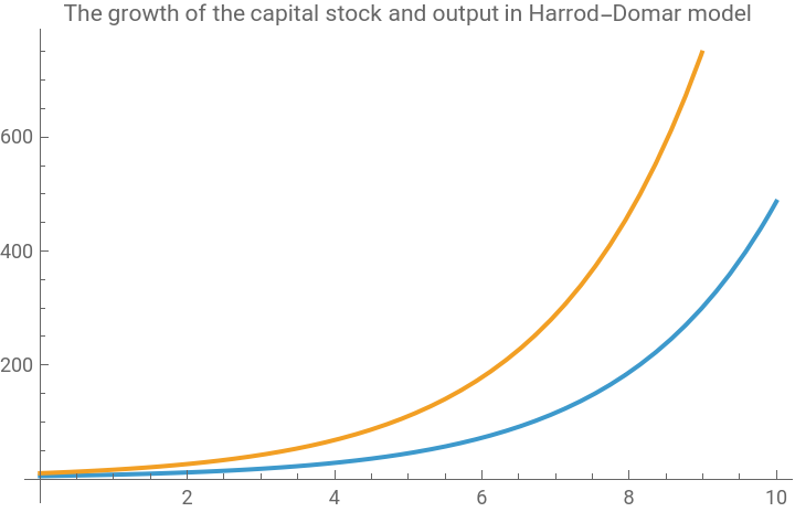
One way of visualizing the solution path is to assign some arbitrary values to the parameters and determine the unique solution path.
In[]:=
s=0.2;δ=0.02;v=0.4;Y0=10;K0=5;sol2=DSolve[{Y'[t]==(s/v-δ)Y[t],K'[t]==sY[t]-δK[t],Y[0]==Y0,K[0]==K0},{Y[t],K[t]},t]//SimplifyPlot[Evaluate[{K[t],Y[t]}/.sol2],{t,0.`,10.`},PlotLabel->"The growth of the capital stock and output in Harrod-Domar model",PlotLegends->{"K(t)","Y(t)"}]
Out[]=
{{K[t](1.+4.),Y[t]10.}}
-0.02t
0.5t
0.48t
Out[]=
An interactive visualization of solution curves
An interactive visualization of solution curves
Alternatively, we can use the following syntax to create an interactive chart that shows the changing behaviors of the solution curves:
In[]:=
Clear[s,v,δ,Y,PCS,Y0,K0,t,eqn3,sol3];(*Forthisinteractivesimulation,wereplacethenotationforthecapitalstock,K,byPCS*)Y0=10;PCS0=5;δ=0.02;eqn3={{Y'[t]==(s/v-δ)Y[t],PCS'[t]==sY[t]-δPCS[t],Y[0]==Y0,PCS[0]==PCS0}};sol3=ParametricNDSolve[eqn3,{Y,PCS},{t,0,100},{s,v}];ManipulateRowPlotEvaluate[Y[s,v][t]/.sol3],,{t,0,100},PlotLabel->"The warranted vs. actual growth of output",PlotRange->{0,1000000},AxesLabel->{"Time","Y(t)"},PlotStyle->{Blue,{Red,Dashed}},ImageSize->400,Plot[Evaluate[PCS[s,v][t]/.sol3],{t,0,100},PlotLabel->"The growth of the productive capital stock",PlotRange->{0,1000000},PlotStyle->Red,AxesLabel->{"Time","K(t)"},ImageSize->400],Style["Paramters",Bold],{{s,0.07,"Savings rate(s)"},0.05,0.15,ImageSizeTiny,Appearance"Labeled"},{{v,0.5,"Capital-output ratio(v)"},0.3,0.6,ImageSizeTiny,Appearance"Labeled"},SaveDefinitions->True
(0.07/0.5)t
Conclusion
Conclusion
The solution curve for the Harrod-Domar model exhibits an exponential growth of the aggregate output-income and the capital stock. However, depending on the size of parameters, particularly, the savings rate, s, and the capital-output ratio, v, the speed and the shape of the exponential growth curve changes.
For example, given v, the higher saving rate leads to an explosive growth rate of aggregate output-income and the capital stock; while given s, the higher capital-output ratio tends to slow down the speed of the exponential growth pattern of both variables. Only when these two ratios remain a certain stable value, we can anticipate that the model economy will exhibit a sustained and stable exponential growth path.
But what makes the stable and balanced ratio between the savings rate and the capital-output ratio possible? Even if some governments in many newly independent countries at the end of WWII somehow managed to mobilize a higher domestic savings rate for the time being through various economic policies, the same governments could not aim to control the desirable capital-output ratio directly because this ratio was beyond the policy target. The actual economic growth pattern, therefore, must exhibit an alternate cycle of explosive growth followed by a slower accumulation of the capital stock, which was induced by imbalances between savings rate and the capital-output ratio.
Notice also that there is no labor market variable in this model. If we introduce a certain capital-labor ratio, similar to the capital-output ratio, we may be able to develop the original Harrod-Domar model further to account for the changing demand for labor given a certain growth of civilian labor force. In this case, however, we cannot infer any optimistic conclusion about the full employment of labor in the labor market because there is no guarantee that the labor supply adjusts fast enough to the changing demand for it, the latter of which is determined by the changing ratio between savings rate and the capital-output ratio. This ‘business cycle’ prone ‘under-employment’ feature of economic growth process is a stark contrast to many neoclassical economic growth models that would come later.
Reference
Reference
◼
Evsey D. Domar, “Capital Expansion, Rate of Growth, and Employment,” Econometrica, April 1946, pp.137-147 (reprinted in Domar, Essays in the Theory of Economic Growth, Oxford University Press, 1957, pp.70-82)
◼
Alpha C. Chiang and Kevin Wainwright, Fundamental Methods of Mathematical Economics, McGraw Hill: 2005 (the fourth edition), pp.471-474.
CITE THIS NOTEBOOK
CITE THIS NOTEBOOK
Introduction to dynamic economic models: the Harrod-Domar growth model
by Hee-Young Shin
Wolfram Community, STAFF PICKS, January 6, 2026
https://community.wolfram.com/groups/-/m/t/3602119
by Hee-Young Shin
Wolfram Community, STAFF PICKS, January 6, 2026
https://community.wolfram.com/groups/-/m/t/3602119