This project discusses predator - prey system, particularly the Lotka - Volterra equations, which model the interaction between two species : prey and predators . Let' s solve the Lotka - Volterra equations numerically and visualize the results .
Define the parameters
parameters={α->1.0,β->0.1,γ->1.5,δ->0.075};
Define the system of differential equations
equations={x'[t]==αx[t]-βx[t]y[t],y'[t]==δx[t]y[t]-γy[t],x[0]==40,(*initialnumberofprey*)y[0]==9(*initialnumberofpredators*)}/.parameters;
Solve the system
solution=NDSolve[equations,{x,y},{t,0,100}];
Plot the solution over time
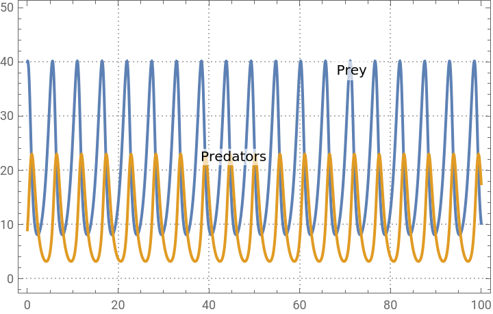
timeSeriesPlot=Plot[Evaluate[{x[t],y[t]}/.solution],{t,0,100},PlotLegends->{"Prey","Predators"},PlotLabels->Placed[{"Prey","Predators"},Above],AxesLabel->{"Time","Population"},PlotTheme->"Detailed"]
Out[]=


Extract the solution for x and y
preySolution=x/.solution[[1]];predatorSolution=y/.solution[[1]];
Define the vector field
vectorField=VectorPlot[{αx-βxy,δxy-γy}/.parameters,{x,0,80},{y,0,30},VectorScale->{Small,Automatic,None},StreamStyle->Red,VectorStyle->Blue];
Solve for equilibrium points
equilibriumPoints=Solve[{αx-βxy==0,δxy-γy==0}/.parameters,{x,y}]

Out[]=
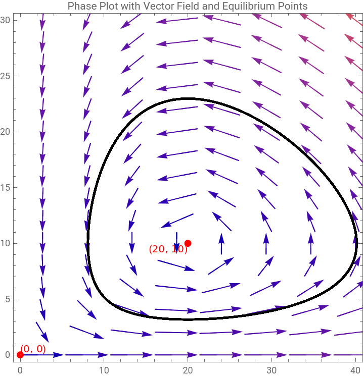
{{x0.,y0.},{x20.,y10.}}
Equilibrium points
equilibriumPoints={{0,0},{20,10}};
Create the phase plot with the vector field and equilibrium points
phasePlotWithVectorField=Show[vectorField,ParametricPlot[Evaluate[{preySolution[t],predatorSolution[t]}],{t,0,100},PlotStyle->{Thick,Black}],Graphics[{Red,PointSize[Large],Point[equilibriumPoints],Text["(0, 0)",{0,0},{-1,-1}],Text["(20, 10)",{20,10},{1,1}]}],AxesLabel->{"Prey Population","Predator Population"},PlotLabel->"Phase Plot with Vector Field and Equilibrium Points",PlotRange->{{0,40},{0,30}},PlotTheme->"Detailed"]
Out[]=
In[]:=
Clear["Global`*"]
Now, we need to handle a modified version of the Lotka - Volterra equations . These modified equations incorporate logistic growth for the prey population . These equations are :αX1--βXYδXY-γY
dX
dt
X
K
dY
dt
Define the parameters
parameters={α->1.0,β->0.1,γ->1.5,δ->0.075,k->100};
Define the system of differential equations
equations={x'[t]==αx[t](1-x[t]/k)-βx[t]y[t],y'[t]==δx[t]y[t]-γy[t],x[0]==40,(*initialnumberofprey*)y[0]==9(*initialnumberofpredators*)}/.parameters;
Solve the system
solution=NDSolve[equations,{x,y},{t,0,100}];
Plot the solution over time
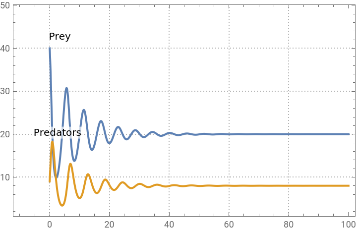
timeSeriesPlot=Plot[Evaluate[{x[t],y[t]}/.solution],{t,0,100},PlotLegends->{"Prey","Predators"},PlotLabels->Placed[{"Prey","Predators"},Above],AxesLabel->{"Time","Population"},PlotTheme->"Detailed"]
Out[]=
Extract the solution for x and y
preySolution=x/.solution[[1]];predatorSolution=y/.solution[[1]];
Define the vector field
vectorField=VectorPlot[{αx(1-x/k)-βxy,δxy-γy}/.parameters,{x,0,120},{y,0,40},VectorScale->{Small,Automatic,None},StreamStyle->Red,VectorStyle->Blue];
Find the equilibrium points
equilibriumPoints=Solve[{αx(1-x/k)-βxy==0,δxy-γy==0}/.parameters,{x,y}];
equilibriumPointsValues=equilibriumPoints/.{x->xval_,y->yval_}:>{xval,yval}
Create the phase plot with the vector field and equilibrium points
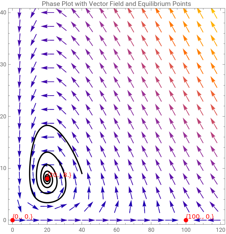
phasePlotWithVectorField=Show[vectorField,ParametricPlot[Evaluate[{preySolution[t],predatorSolution[t]}],{t,0,100},PlotStyle->{Thick,Black}],Graphics[{Red,PointSize[Large],Point[equilibriumPointsValues],Text[ToString[#],#,{-1,-1}]&/@equilibriumPointsValues}],AxesLabel->{"Prey Population","Predator Population"},PlotLabel->"Phase Plot with Vector Field and Equilibrium Points",PlotRange->{{0,120},{0,40}},PlotTheme->"Detailed"]
Out[]=
{{20.,8.},{100.,0.},{0.,0.}}
Out[]=
CITE THIS NOTEBOOK
CITE THIS NOTEBOOK
Standard and extended Lotka-Volterra models with carrying capacity
by Athanasios Paraskevopoulos
Wolfram Community, STAFF PICKS, August 5, 2024
https://community.wolfram.com/groups/-/m/t/3240982
by Athanasios Paraskevopoulos
Wolfram Community, STAFF PICKS, August 5, 2024
https://community.wolfram.com/groups/-/m/t/3240982