The aim of this project is to explore the trivalent networks generated by random replacements using rewriting rules from the Wolfram model. The aim is to connect this to scalar field theory. In the limit of large n, the SU(n) internal symmetry is dominated by Feynman diagrams that exhibit the structure of planar trivalent networks. Hence, the enumeration of trivalent planar graphs play a crucial role in understanding Feynman diagrams for such theory. By applying simple rules iteratively, we can generate complex network structures and examine their emergent behavior in terms of network connectivity and average statistical properties. This research contributes to a deeper understanding of the theory and provides insights into the dynamics of these computational systems.
3
φ
3
φ
Introduction
Introduction
Network analysis is a powerful tool that provides us with a fruitful framework to describe phenomena related to social, technological, and many other real-world complex systems. A simple network system belongs to the host network configuration that allows information and information exchange between several devices. Network rewrite systems provide a framework for investigating the behavior and dynamics of complex networks. In the context of theory, it is important to deal with the principles and systems of these systems, especially physics. Trivalent networks play an important role in the scalar field as it prepares the structure of Feynman diagrams. The relationships of subatomic particles can be complex and difficult to understand intuitively and the Feynman diagrams allow for a simple representation of the rather mysterious abstract formula. In theoretical physics, Feynman diagrams are diagrammatic representations of mathematical expressions.What does the Feynman graph corresponding to the theory look like?
3
ϕ
3
ϕ
3
ϕ
In[]:=
PacletInstall["WolframInstitute/Hypergraph"]
Out[]=
PacletObject

In[]:=
<<WolframInstitute`Hypergraph`
In[]:=
RulePlot[ResourceFunction["WolframModel"][{{x,y},{x,z},{x,w}}->{{x,y},{x,z},{x,w},{y,e},{y,d},{z,r},{z,f},{w,m},{w,n}}]]
Out[]=
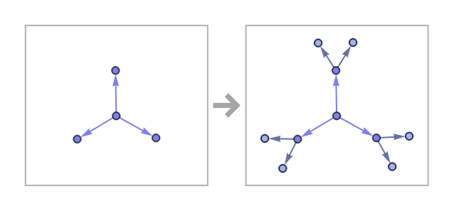
Simple Network Rewriting Systems are a powerful analytical tool for understanding the behavior and dynamics of complex networks. In these systems, the structure and components of a network are guided by specific rewriting rules or transformation functions, leading to changes in the nodes and edges of the network through interactions between them.
Random replacements in network systems
Random replacements in network systems
Random replacements plays a crucial role in network systems and has various applications. Random replacements allows for the exploration of various network properties and phenomena. By generating random networks and analyzing their properties, we can gain insights into the behavior of complex networks.
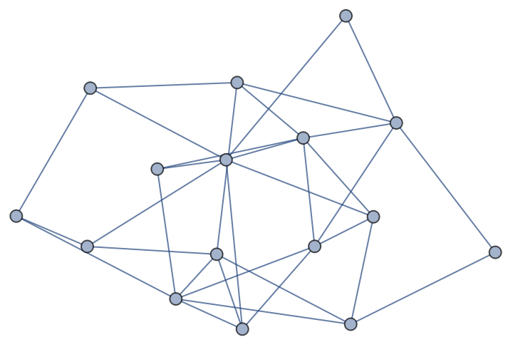
Using the RandomGraph function, we can set up network system with the vertex and edge we have determined.
Using the RandomGraph function, we can set up network system with the vertex and edge we have determined.
In[]:=
RandomGraph[BernoulliGraphDistribution[16,20/(10*(10-1))],VertexSizeMedium]
Out[]=
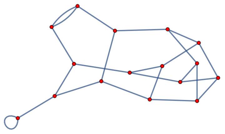
By using the RandomNetwork function, we can generate a random network as an initial configuration . This random network can serve as the starting point for applying the transformation rules of the simple network rewriting systems. The application of these rules to the initial network can lead to further changes in the network structure and dynamics. By studying how the generated random network evolves under the influence of the transformation rules, we can gain insights into the behavior and properties of simple network rewriting systems. This analysis can help us understand how different initial configurations can lead to different network dynamics and explore the emergent patterns and properties of the system.
In[]:=
RandomNetwork[n_?EvenQ]:=Partition[Fold[Insert[#1,#2,Random[Integer,Length[#1]]+1]&,{},Floor[Range[1,n+2/3,1/3]]],2]
In[]:=
RandomNetwork[24]
Out[]=
{{13,11},{9,22},{13,23},{16,17},{6,9},{15,1},{18,1},{12,21},{1,23},{7,11},{3,19},{7,2},{23,17},{14,17},{5,22},{8,4},{24,5},{20,24},{2,9},{14,15},{11,4},{6,19},{22,24},{3,6},{7,10},{2,4},{18,12},{8,21},{12,20},{3,8},{16,20},{14,19},{16,10},{13,10},{18,21},{5,15}}
In[]:=
Graph[RandomNetwork[16],VertexStyleRed,EdgeStyle->Thick]
Out[]=
Node Importance and Centrality Measures:
Node Importance and Centrality Measures:
The importance of a node within a network can be determined by various centrality measures. These measures capture different aspects of a node’s position within the network structure and can provide insights into the node’s influence, reachability, or contribution to the network’s connectivity.
In[]:=
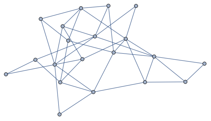
g=RandomGraph[{20,40}]degrees=VertexDegree[g]closeness=ClosenessCentrality[g]betweenness=BetweennessCentrality[g]eigenvector=EigenvectorCentrality[g]pagerank=PageRankCentrality[g]
Out[]=
Out[]=
{5,3,5,5,6,7,2,2,4,2,3,2,6,4,3,4,3,4,4,6}
Out[]=
{0.527778,0.44186,0.527778,0.487179,0.542857,0.575758,0.395833,0.358491,0.5,0.431818,0.387755,0.413043,0.575758,0.463415,0.452381,0.513514,0.44186,0.475,0.475,0.527778}
Out[]=
{15.6786,3.64286,19.3429,10.6286,22.7048,31.6952,1.16667,0.,4.04286,0.833333,1.25,0.,33.0357,6.9119,2.67857,6.92619,6.61667,9.90952,8.67619,30.2595}
Out[]=
{0.0668913,0.0406586,0.0604151,0.0593768,0.0763245,0.0759482,0.0237721,0.0236203,0.058458,0.0326465,0.0334927,0.0304212,0.0700137,0.0469272,0.0437884,0.0566994,0.0306103,0.0541255,0.0434248,0.0723854}
Out[]=
{0.0594687,0.0384107,0.0610229,0.0600207,0.0708366,0.0840971,0.0293059,0.0293373,0.0485477,0.0278066,0.0408131,0.0280857,0.0725043,0.0493902,0.0380846,0.0487573,0.0409204,0.0497464,0.0503243,0.0725195}
Networks that generating arbitrary transformations
Networks that generating arbitrary transformations
In the context of network analysis, generating arbitrary transformations between networks refers to the process of creating mappings or transformations that convert one network into another while preserving certain properties or relationships. In Wolfram Mathematica, there are several functions and techniques available to generate such transformations between networks.
In[]:=
networkFunction[n_Integer]:=Module[{g,g1,g2},g=Graph3D[{1,2,3,4},{1->3,3->2,2->1,1->4,2->4,3->4}];g1=Graph3D[{1,2,3,4},{1->3,3->2,2->1,3->4}];g2=EdgeAdd[g1,{45,56,61,52,64}];Which[n==1,g,n==2,g1,n==3,g2,True,"Invalid input"]]
In[]:=
networkFunction[1]networkFunction[3]
Out[]=

Out[]=

The networkFunction function in the provided code defines a network system with three different states or configurations represented by graphs g, g1, and g2. The function takes an input n to determine which state or configuration to return. In the context of a network system, each graph represents a specific arrangement of nodes and edges, which can correspond to various components and connections within a real-world network. The networkFunction function can be seen as a simplified model of a network system with three distinct configurations.
By utilizing the WolframModel resource function, we can define rules for transforming network structures and visualize their evolution using RulePlot. This section demonstrates the usage of these functions to analyze the evolution of a specific network rule. Let' s consider an example using the rule defined by the expression:
In[]:=
rule=ResourceFunction["WolframModel"][{{1,2},{1,3},{1,4}}->{{5,6},{6,7},{5,7},{2,5},{3,6},{4,7}}];
To visualize the evolution of a network structure according to this rule, we can use the following function:
In[]:=
RulePlot[rule=ResourceFunction["WolframModel"][{{1,2},{1,3},{1,4}}->{{5,6},{6,7},{5,7},{2,5},{3,6},{4,7}}]]
Out[]=
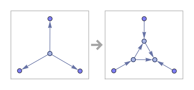
This code generates a plot illustrating the step-by-step transformation of the initial network structure {{1, 2}, {1, 3}, {1, 4}, {2, 3}, {3, 4}, {2, 4}} according to the specified rule. To further analyze the resulting network structures, we can use GraphPlot3D. The following function demonstrates this by visualizing the network structures at different evolution steps:
In[]:=
GraphPlot3D[UndirectedEdge@@@#,GraphLayout->"SphericalEmbedding"]&/@ResourceFunction["WolframModel"][{{1,2},{1,3},{1,4}}->{{5,6},{6,7},{5,7},{2,5},{3,6},{4,7}},{{1,2},{1,3},{1,4},{2,3},{3,4},{2,4}},8,"StatesList"]
This function generates a sequence of 3D network visualizations corresponding to different steps in the evolution of the initial network structure, according to the specified rule. Each network structure is represented by a set of undirected edges, obtained from the evolution process.
Consider the following transformation rule T1, implemented in Mathematica:
This rule can be applied to an initial graph, such as a hexagonal grid:
We can transform a planar network to another network with the same node arrangement.
The transformation rule is applied using the ruleApply function, and we can generate a sequence of transformed graphs using NestList function:
After 50,100 and 500 steps, it looks like ...
Diameters of these graphs can be calculated using the GraphDiameter function:
Finally, the sequence of diameters can be plotted to provide a visualization of the changing network properties :
This process demonstrates how network dynamics can be modeled and analyzed using transformation rules and graph theory, with parallels to the process of studying interactions in quantum field theory.
Now let’s look at the average of the number of edges of the hexagonal graph. Faces are identified using the PolyhedralGraphFaces resource function. Each face represents a closed loop in the graph, and the total number of faces and the number of edges of each face are calculated.
Due to evaluation time constraint, we consider here a small version of the above graph.
After 10 steps of applying rewriting rules, it transforms into the following.
Counting number of vertices in the above graph:
Counting number of edges in the above graph:
Identifying the faces in the above graph:
Finding the coordinates of those faces:
Finding the number of edges for all the identified faces:
Eliminating the last sub-list corresponding to the entire graph (trivial case):
Average number of faces:
The average number of edges per face is approximately 6.
Concluding remarks
Concluding remarks
Keywords
Keywords
◼
Trivalent Network
◼
Rewriting Rules
◼
Wolfram Model
Acknowledgment
Acknowledgment
I would like to extend my gratitude to Stephen Wolfram for suggesting the idea of studying behaviour of simple network rewriting systems. I would like thank my mentors Adiba Shaikh and Nikolay Murzin for their time and guidance. Their advice, suggestions and coding help were invaluable. Finally, I want to thank everyone who made Wolfram Summer School possible.
References
References
CITE THIS NOTEBOOK
CITE THIS NOTEBOOK
Studying behavior of simple network rewriting system
by Minaya Allahverdiyeva
Wolfram Community, STAFF PICKS, July 12, 2023
https://community.wolfram.com/groups/-/m/t/2959571
by Minaya Allahverdiyeva
Wolfram Community, STAFF PICKS, July 12, 2023
https://community.wolfram.com/groups/-/m/t/2959571