Cryptocurrency price prediction with recurrent neural networks
by Shivay Nagpal
St. Stephen's College, University of Delhi
by Shivay Nagpal
St. Stephen's College, University of Delhi
Deep learning is becoming commonplace in many fields of the financial world. The ability to identify and predict patterns in large data sets is a powerful tool which can be deployed in making various kinds of predictions. Since the Cryptocurrency market is considered to be very dynamic and complex in nature, this project aims to use a Long short-term memory (LSTM) Recurrent Neural Network (RNN) to make short term predictions of the values of various popular cryptocurrencies using the Wolfram Language. The dataset we will use for this project includes market values for three popular cryptocurrencies on the market.
A time series is a sequence of data points of that occur in successive order over some period of time. In this project, we have trained three different Long Short-term Memory (LSTM) Recurrent Neural Networks(RNNs) with historical data of the market values of three popular cryptocurrencies. These neural networks will then be employed to make predictions on the time-series that will then be compared with the real dataset with various statistical parameters.
Wrangling and Exploring the Data
Wrangling and Exploring the Data
Creating TimeSeries of our primary data
Creating TimeSeries of our primary data
We will begin by making Time-series of the market values of three popular cryptocurrencies of the world, namely Bitcoin (BTC), Ethereum (ETH) and Litecoin (LTC) using a Resource Function from the Wolfram repository to obtain this data.
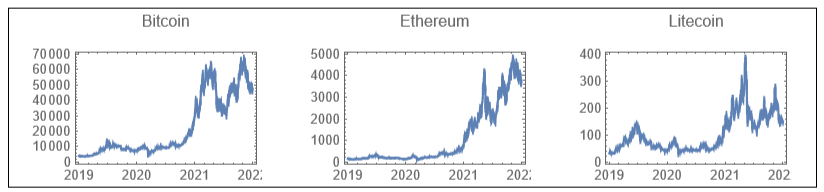
Creating three Time-series containing market values of the cryptocurrencies from the year 2019 to 2022:
In[]:=
btc=TimeSeriesWindow[ResourceFunction["https://www.wolframcloud.com/obj/antononcube/DeployedResources/Function/CryptocurrencyData"]["BTC"],{{2019,1,1},{2022,1,1}}];eth=TimeSeriesWindow[ResourceFunction["https://www.wolframcloud.com/obj/antononcube/DeployedResources/Function/CryptocurrencyData"]["ETH"],{{2019,1,1},{2022,1,1}}];ltc=TimeSeriesWindow[ResourceFunction["https://www.wolframcloud.com/obj/antononcube/DeployedResources/Function/CryptocurrencyData"]["LTC"],{{2019,1,1},{2022,1,1}}];
It is worth noticing that the data obtained includes values from 2020, an year which saw the COVID-19 crisis which caused severe market volatility and regular pattern deviation.
Visualising the obtained data:
Out[]=
Preparing the data for training the Neural Networks
Preparing the data for training the Neural Networks
To prepare our data for training the neural networks, we will first employ the Augmented Dickey-Fuller (ADF) Test to check for the Stationarity of the time-series. Since a stationary time series has no autocorrelation in the errors, it provides a considerable improvement in eventual forecasting performance.
The ADF test returns the probability of the null hypothesis which supports the existence of a unit root.
The ADF test returns the probability of the null hypothesis which supports the existence of a unit root.
Applying ADF test to check for stationarity on our original time-series:
Applying ADF test to check for stationarity on our original time-series:
Out[]=
p-Value of Null Hypothesis | ||
BTC | ETH | LTC |
0.805144 | 0.912751 | 0.378303 |
As we can observe, these values are significantly high and the existence of a unit root is likely. Consequently, our time-series are non-stationary and is unsuitable to be directly used to train our neural networks. To improve the normality of our data, we will use a Box-Cox transformation with λ=0 (Logarithmic transformation) on all of our time-series.
Transforming the time-series
Transforming the time-series
Applying Logarithmic Transformation to the timeseries:
Applying Logarithmic Transformation to the timeseries:
In[]:=
transformedbtc=Log/@btc["Values"];transformedeth=Log/@eth["Values"];transformedltc=Log/@ltc["Values"];
We will evaluate the stationarity and visualise the differences of these transformed time-series:
Applying ADF Test to the differences of the transformed time-series:
Out[]=
p-Value of Null Hypothesis | ||
BTC | ETH | LTC |
9.73386× -18 10 | 8.5833× -18 10 | 1.1745× -17 10 |
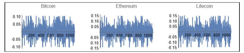
As we can observe, the differences of the transformed data return very small p-Values for the Null hypothesis supporting the existence of the unit root and can be considered stationary, and hence are suitable for training our Neural Networks.
Visualising the differences of the transformed data:
Out[]=
Now we need to make partitions of the data that we can feed to our Neural Networks to train them, but before we can do that, we need to determine the size of these partitions, or the lag of the training data. The lag can be assumed to be three under the assumption that differencing of order higher than three would be extremely unlikely for any time-series.
Preparing data for training the neural network:
Preparing data for training the neural network:
Now, we will create associations that will take three consecutive values from the time series and associate it with the adjacent fourth value. This is then repeated for all the cryptocurrencies.
Functions creating associations from the data for training the neural network:
In[]:=
lag=3;btcData=Most[#]Last[#]&/@(Partition[transformedbtc,lag+1,1]);ethData=Most[#]Last[#]&/@(Partition[transformedeth,lag+1,1]);ltcData=Most[#]Last[#]&/@(Partition[transformedltc,lag+1,1]);
We then split the data so that 90% is used for training the Neural Networks and the remaining 10% is used for testing.
Splitting the data as training and testing sets:
In[]:=
frac=Ceiling[Length[btcData]*0.9];{btctrain,btctest}={btcData[[;;frac]],btcData[[frac+1;;]]};{ethtrain,ethtest}={ethData[[;;frac]],ethData[[frac+1;;]]};{ltctrain,ltctest}={ltcData[[;;frac]],ltcData[[frac+1;;]]};
Here, we have taken the initial 985 (90%) data points and made training data sets for all our cryptocurrencies. Further, 109 (10%) data points have been assigned to the individual cryptocurrencies’ testing sets.
Neural Net Model trained with one cryptocurrency:
Neural Net Model trained with one cryptocurrency:
The first model uses a 10 layered LSTM neural network. It can be trained on data of individual cryptocurrencies that we prepared above.
Defining the network:
Out[]=
NetChain


Training the model on Bitcoin data with 300 training rounds:
In[]:=
btctrained1=NetTrain[model1,btctrain,ValidationSetbtctest,MaxTrainingRounds300]
Out[]=
NetChain

Similarly, training the model on Ethereum and Litecoin data with 300 training rounds each :
In[]:=
ethtrained1=NetTrain[model1,ethtrain,ValidationSetethtest,MaxTrainingRounds300];ltctrained1=NetTrain[model1,ltctrain,ValidationSetltctest,MaxTrainingRounds300];
Now we will use our three trained networks to predict the Box-Cox transformed values of the currencies they were trained on over their respective testing sets.
Creating lists of predicted values:
In[]:=
predictedbtc1=btctrained1[Keys[btctest]];predictedeth1=ethtrained1[Keys[ethtest]];predictedltc1=ltctrained1[Keys[ltctest]];
This chart summarises the statistical parameters that describe the predicted data compared to the real test data:
Out[]=
Prediction Parameters | |||
RSquared | MeanSquare | StandardDeviation | |
Bitcoin | 0.864537 | 0.00241482 | 0.0491408 |
Ethereum | 0.855202 | 0.0025003 | 0.050003 |
Litecoin | 0.884982 | 0.00301313 | 0.0548919 |
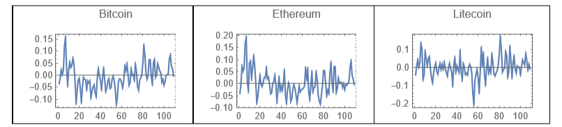
The p-Values of the null hypothesis stating that the residuals for each cryptocurrency are random are also calculated.
Creating a p-Value table:
Out[]=
p-Values | ||
Bitcoin | Ethereum | Litecoin |
4.57336× -13 10 | 2.9141× -7 10 | 0.000573151 |
Visualising the residuals for each cryptocurrency:
Out[]=
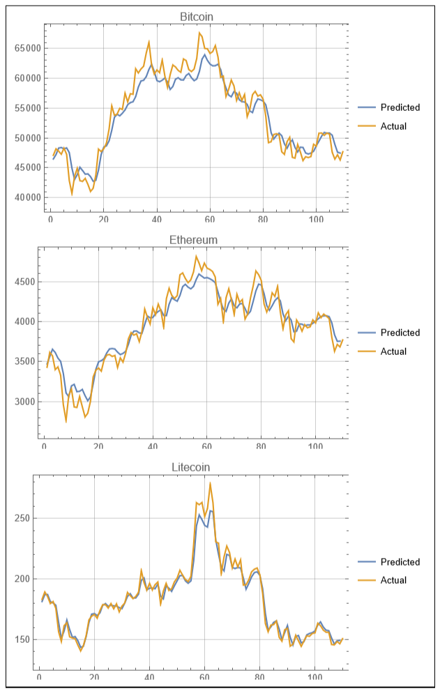
Since we applied a Box-Cox (Logarithmic) transformation to our data initially, we will use a reverse exponential transformation to obtain the predicted market values of the cryptocurrencies:
Applying exponential transformation to our predicted data:
In[]:=
predictedbtctransformed1=Exp/@predictedbtc1;predictedethtransformed1=Exp/@predictedeth1;predictedltctransformed1=Exp/@predictedltc1;
Visualising the predicted market values against the real data:
Out[]=
Alternate Neural Net Model trained with one cryptocurrency:
Alternate Neural Net Model trained with one cryptocurrency:
The second model also uses a 10 layered LSTM neural network. It differs from the first model as it has a higher dropout in its dropout layer that makes each layer less sensitive to extreme statistical fluctuations. It is also capable of being trained on a single cryptocurrency’s data like our first model.
Defining the network:
Training the model on individual cryptocurrencies’ data separately for 300 rounds each:
Now we will use our three trained networks to predict the Box-Cox transformed values of the currencies they were trained on over their respective testing sets:
Creating lists of predicted values:
This chart summarises the statistical parameters that describe the predicted data compared to the real test data:
The p - Values of the null hypothesis stating that the residuals for each cryptocurrency are random are also calculated.
Creating a p-Value table:
Visualising the residuals for each cryptocurrency :
Now we will apply an inverse logarithmic (exponential) transformation to our data like we did in the previous model.
Applying exponential transformation to our predicted data:
Visualising the predicted market values against the real data:
Neural Net Model trained with 3 Cryptocurrencies:
Neural Net Model trained with 3 Cryptocurrencies:
Since the market value of cryptocurrencies might have some interdependence, the third model that we will use here will be trained on all three cryptocurrencies together, but will predict the values of only one cryptocurrency as output. Hence, we will have to train it thrice over all cryptocurrencies so that the network learns how fluctuations in all the currencies’ value affect the one that it is tasked with predicting.
Defining the pre-concatenation chain of the network:
Defining the post-concatenation chain of the network:
Defining the entire neural network:
Preparing data for training the neural network:
Preparing data for training the neural network:
Now, we will create associations that will take three consecutive values from all three time series and associate it with the adjacent fourth value of a particular cryptocurrency. This is then repeated for all the cryptocurrencies. We will also split the data as training (90%) and test (10%) sets.
Functions creating associations from the data for training the neural network:
Training the model on individual cryptocurrencies’ data separately for 300 rounds each:
We will employ these three trained networks to predict values of the currencies they were trained for:
Creating lists of predicted values:
This chart summarises the statistical parameters that describe the predicted data compared to the real test data:
The p - Values of the null hypothesis stating that the residuals for each cryptocurrency are random are also calculated.
Creating a p-Value table:
Visualising the residuals for each cryptocurrency :
Now we will apply an inverse logarithmic (exponential) transformation to our data like we did in the previous models
Applying exponential transformation to our predicted data:
Visualising the predicted market values against the real data:
Concluding remarks
Concluding remarks
In this project, we conducted an experimental analysis using significant amounts of cryptocurrency data from three very popular cryptocurrencies of the world, namely Bitcoin(BTC), Ethereum(ETH) and Litecoin(LTC). The models that were used varied significantly from each other as the first two exclusively used the past data of the cryptocurrency they were tasked with predicting, independent of the other cryptocurrencies. The third model was slightly more complex as it operated on multi-input architecture, and was trained to evaluate how all three currencies affect the prices of each other.
All three models were fairly accurate in their capability to predict the price of the cryptocurrencies, though the third model with the multi-input architecture developed a forecasting model with the best regression. It is worth noting that although the regression metrics appear similar between the second model and the third model, the third (multi-input architecture) model consistently outperformed the other models through various rounds of training.
The analyses also shows that the proposed models are efficient in dealing with mixed cryptocurrency data with low computation costs.
Since the results are fairly encouraging, the models can be further extended to be trained on more cryptocurrencies, which can tell us about sets of cryptocurrencies that are more correlated to each other and can also include more financial technical indicators like volume of transactions and daily high and low prices to make even more accurate predictions.
All three models were fairly accurate in their capability to predict the price of the cryptocurrencies, though the third model with the multi-input architecture developed a forecasting model with the best regression. It is worth noting that although the regression metrics appear similar between the second model and the third model, the third (multi-input architecture) model consistently outperformed the other models through various rounds of training.
The analyses also shows that the proposed models are efficient in dealing with mixed cryptocurrency data with low computation costs.
Since the results are fairly encouraging, the models can be further extended to be trained on more cryptocurrencies, which can tell us about sets of cryptocurrencies that are more correlated to each other and can also include more financial technical indicators like volume of transactions and daily high and low prices to make even more accurate predictions.
Keywords
Keywords
◼
Time-series Forecasting
◼
Recurrent neural network
◼
Deep Learning
◼
Long Short-Term Memory (LSTM)
◼
Cryptocurrency Prediction
Acknowledgment
Acknowledgment
I am deeply thankful to my mentor, Siria Sadeddin for her invaluable guidance and support that she provided me with throughout the duration of Wolfram India School 2022. This project would not have been remotely feasible without her constant assistance and insights. I am also thankful to the Wolfram India School Team, especially Tuseeta and Mads, for conducting the school with utmost precision amid these challenging times.
References
References
◼
Livieris, I.E.; Kiriakidou, N.; Stavroyiannis, S.; Pintelas, P. An Advanced CNN-LSTM Model for Cryptocurrency Forecasting. Electronics 2021, 10, 287. https://doi.org/10.3390/electronics10030287
◼
Livieris, I.E.; Stavroyiannis, S.; Pintelas, E.; Pintelas, P. A novel validation framework to enhance deep learning models in
time-series forecasting. Neural Comput. Appl. 2020, 32, 17149–17167.https://doi.org/10.1007/s00521-020-05169-y
time-series forecasting. Neural Comput. Appl. 2020, 32, 17149–17167.https://doi.org/10.1007/s00521-020-05169-y
◼
Anton Antonov, Crypto-currencies data acquisition with visualization, (2021), MathematicaForPrediction at WordPress.