Wolfram mathematica . . .How to solve typical mathematics textbook problems on the most advanced computer algebra system in the world. Roger Wells July 2023{“Kernel” -> {“Version” -> “11.2.0 for Microsoft Windows (64-bit) (September 11, 2017)”, “ReleaseID” -> “11.2.0.0 (5822651, 2017091101)”, “LicenseID” -> “L3991-4623”, “PatchLevel” -> “0”, “ActivationKey” -> “3991-4623-49AQHW”, “ActivationGroupID” -> “L3991-4623”, “MachineID” -> “6202-12511-69189”, “UserName” -> “Owner”, “MachineName” -> “tyrannasaurus-r”, “MachineDomains” -> {}, “LicenseServer” -> “tyrannasaurus-r”, “MaxLicenseProcesses” -> 2, “LicenseExpirationDate” -> {Infinity, 0, 0, 0, 0, 0}, “MachineType” -> “PC”, “OperatingSystem” -> “Windows”, “ProcessorType” -> “x86-64”, “Language” -> “English”, “CharacterEncoding” -> “WindowsANSI”, “SystemCharacterEncoding” -> “WindowsANSI”, “TimeZone” -> -6., “CreationDate” -> DateObject[{2017, 9, 11, 10, 31, 25.}, “Instant”, “Gregorian”, -6.], “InstallationDirectory” -> “C:\\Program Files\\Wolfram Research\\Mathematica\\11.2”,Machine Epsilon 2022045 * 10^-16 Machine precision 159546 Machine Number Limits { 2.225.7 * 10^ -308, 1,79769 *10^ 308} Number Limits {6,22968849675322 * , 16052167619336622 * } This is an active computable document created on software owned by Roger Wells January 2018 . Wolfram Mathematica ID: rogerwells2017@hotmail.com. PTC Mathcad username: iornfist666@yahoo.com Password: Javadog License Number 3991-4623 Password: 1javadog Mathcad serial # EN901002DS2411A https://user.wolfram.com/portal/ProductRegistration?execution=e1s Linkdln: fgmju@yahoo.com 1javadog!Quadratic EquationSolve for X + b(x) +c = 0
Matrix Algebra Parenthesis to open Matrix ()control + enter = Rowcontrol + comma = Column
The input (above) is Matrix Form (obviously). The software considers this to be a Graphic (picture)The output (below) is a List of Lists. This is available to be used as input for computation Assign these variables, then use them in a MatrixDifferential CalculusDetermine the general solution. = Note the output is again a List with two arguments {{ x→ neg} , {x→pos}}In the Wolfram language = [ X ] y = [ X ] Y = Y [ x ] ( keeping Y as a function of X )Determine the second order general solution. xy - 2 - 8y = 0 yx = - 2 - 8y = 0Specific solutions and boundary conditions . . .DSolve[ { x’ [ t ] = = [ t ], x [ 0 ] = = }, x [ t ] , t ] Elementary displacement function f (x.) initial value zeroDetermine the general solution of the differential equation = k ( y - T )Assume the initial conditions Y(0) = T1A typical population growth model where T and T1 are (time ( 0 ) and time (1) ) “initial value and condition”Wolfram mathematica . . . DSolve [ { y ’ [ x ] = = k ( y [ x ] - T ) , y [ 0 ] = = T1 } , y [ x ], x ]DSolve [ { y’ [ x ] k ( y [ x ] - T ) , y [ 0 ] T1 } , y [ x ] , x ] note the space between k * (the constant) and k * ( y [ x ] - T ) multiplication implied Mathematica returns the output NDSolve[{y’[x] == Sin[y[x]], y[0] == 1}, y, {x, 0, 4}] With NDSolve the “interpolating” function appears.The windows can also be opened and contain a wealth of information and algorithms pertaining to the differential equation. % 1 [ [1, 1, 2] ] This now uses % which means input from last line (1).Calculus II modeling homework answers to precisely match textbook pictures.Filling from the 2 plot, (the second in the list of functions), to→3 the number three function,2x),don’t forget to {3}.
-1355718576299610
10
1355718576299609
10
2
a(x)
Solve[ax^2+bx+c0,x]
x,x
-b--4ac
2
b
2a
-b+-4ac
2
b
2a
MatrixFormx,x
-b--4ac
2
b
2a
-b+-4ac
2
b
2a
x -b- 2 b 2a |
x -b+ 2 b 2a |
Solve[ax^2+bx+c0,b]
b
-c-a
2
x
x
Solve[ax^2+bx+c0,c]
{{c-bx-a}}
2
x
| | | |
| | | |
| | | |
| | | |
{{,,,},{,,,},{,,,},{,,,}}
a=4;b=3;
c=3;
d=2;
A=
;
a | b |
c | d |
Inv=Inverse[{{a,b},{c,d}}]
{{-2,3},{3,-4}}
MatrixForm,-,-,
d
-bc+ad
b
-bc+ad
c
-bc+ad
a
-bc+ad
-2 | 3 |
3 | -4 |
dy
dx
2x+y
y-x
DSolvey'[x],y[x],xyoumustcompletethearguments...,Y[x],XandclosetheBracet
2x+y[x]
y[x]-x
y[x]x-+3,y[x]x++3
2C[1]
2
x
2C[1]
2
x
Dy
Dx
Y
2
D
2
Dx
''
Y
2
Dy
2
Dx
dy
dx
2
D
2
D
dy
dx
DSolve[y''[x]-2y'[x]-8y[x]==0,y[x],x] remembertousedoubleequalsign
{{y[x]C[1]+C[2]}}
-2x
4x
{{x[t]}}
t
Dy
Dx
{{y[x]T-T+T1}}
kx
kx
yInterpolatingFunctionThesewindowsappearintheanswer.Theyarereadyforcalculationsonthenextline.


InterpolatingFunction

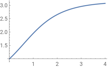
Plot[%2[x.],{x.,0.,4.}]
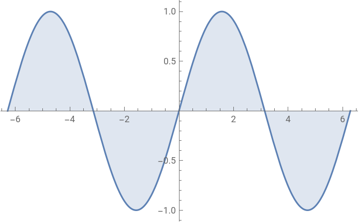
Plot[Sin[x],{x,-2π,2π},FillingAxis]
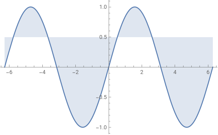
Plot[Sin[x],{x,-2π,2π},Filling->0.5]
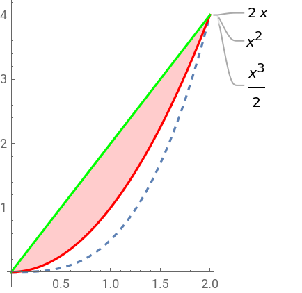
Plot,,2x,{x,0,2},PlotStyle{Dashed,Red,Green},PlotLabelsAutomatic,Filling{2{3}}
3
x
2
2
x
2
x
f[t_,A_,w_,]=A*Sin[w*t]ASin[tw]Manipulate[Plot[ASin[tw],{t,-8,8}],{A,-8,8},{w,-2,2}]

