ABSTRACT (original article): It is shown, how to construct a system of ordinary differential equations of arbitrary order, which has the periodic attractor and models some genetic network of arbitrary size. The construction is carried out by combining of multiple systems of lower dimensions with known periodic attractors. In our example the six-dimensional system is constructed, using two identical three-dimensional systems, which have stable periodic solutions. CITATION (original article): I. Samuilik and F. Sadyrbaev, “Genetic engineering – construction of a network of arbitrary dimension with periodic attractor”, Vibroengineering PROCEDIA, Vol. 46, pp. 67–72, Nov. 2022, https://doi.org/10.21595/vp.2022.22992
Introduction
Introduction
The system we wish to construct, is a special one. It describes the evolution of a network, that consists of elements xi(t), depending on time t. The respective system of ordinary differential equations consist of a nonlinear part and the linear one. Without a nonlinear part solutions of this system exponentially degenerate. The nonlinearity should be similar to the linear function, but bounded, to feet the realities of nature. Sigmoidal functions are good enough. In the text of a notebook the system is visible under the command NDSolve. There are two-dimensional, three-dimensional and even six-dimensional versions. Where from a system of arbitrary dimension arises? A system of arbitrary dimension can be composed of blocks of low dimensions. If any of these blocks has its own periodic solution, the resulting system also has it. The respective trajectory is the curve in the phase space of higher dimension.
Two-dimensional system
Two-dimensional system
Start with the two-dimensional system. The coefficient matrix and the parameters and are specially selected.
W2 = , }, {, }}
{{
α
1
β
1
α
2
β
2
θ
i
μ
i
W=
1 | 1 |
-1 | 0.4 |
{{1,1},{-1,0.4`}}
v1=1;v2=1;
α1=1;β1=1;α2=-1;β2=0.4;μ1=20;μ2=40;Θ1=1;Θ2=-0.3;
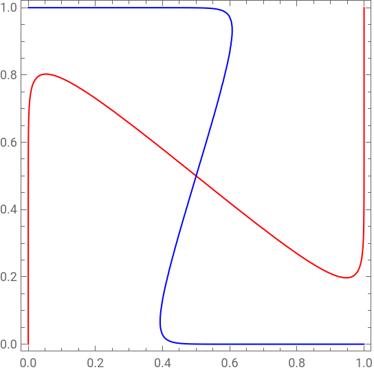
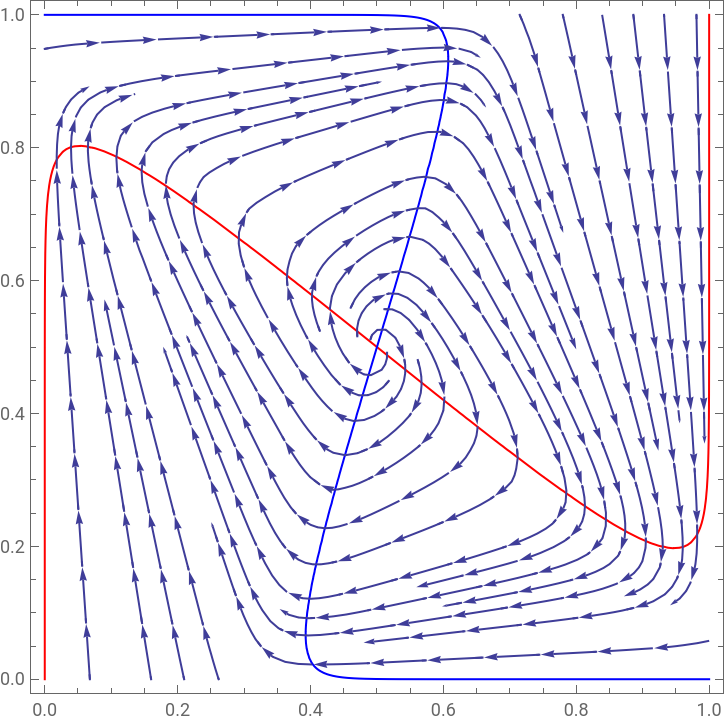
The two nullclines form a framework for desired solution.
uk=ContourPlotx,y,{x,0,1},{y,0,1},ContourStyle{Red,Blue},AxesLabel{x,y}
1
1+
-μ1(α1x+β1y-Θ1)
1
1+
-μ2(α2x+β2y-Θ2)
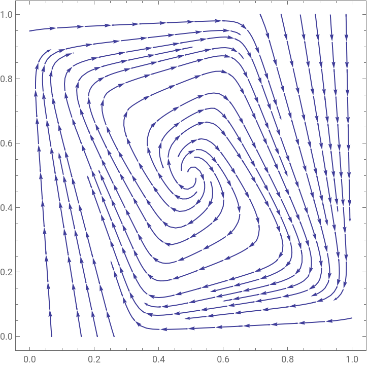
StreamPlot command shows the vector field, that needs to be rotating (whirling).
us=StreamPlot-x,-y,{x,0,1},{y,0,1},StreamPoints20
1
1+
-μ1(α1x+β1y-Θ1)
1
1+
-μ2(α2x+β2y-Θ2)
Show[uk,us]
Critical points
Critical points
Clear[x,y]
FindRoot command confirms that parameters are chosen correctly and the critical point (equilibrium) is located centrally . The type of the central critical point needs to be calculated . For this, the standard linearization process is used . The type of the critical point is unstable focus, and this is the reason why the stable periodic solution emerges . Similar construction can be repeated for the three - dimensional case . To solve the system and visualize the resulting periodic solution is more complicated task .
θ
i
FindRootx==,y==,{{x,0.5},{y,0.5}}
1
v1
1
1+
-μ1(α1x+β1y-Θ1)
1
v2
1
1+
-μ2(α2x+β2y-Θ2)
{x0.5,y0.5}
Calculation of gi
Calculation of
g
i
g1[x0_,y0_]:=;g2[x0_,y0_]:=;
Exp[-μ1(α1x0+β1y0-Θ1)]
2
(1+Exp[-μ1(α1x0+β1y0-Θ1)])
Exp[-μ2(α2x0+β2y0-Θ2)]
2
(1+Exp[-μ2(α2x0+β2y0-Θ2)])
Explore a particular critical point
Explore a particular critical point
x=0.5`;y=0.5`;
G1=g1[x,y]
0.25
G2=g2[x,y]
0.25
Constructing characteristic equation for a particular critical point
Constructing characteristic equation for a particular critical point
B=v1+v2-μ1α1G1-μ2β2G2
-7.
C1=μ1μ2α1β2G1G2-μ1α1G1v2-μ2β2G2v1-μ1μ2α2β1G1G2+v1v2
62.
Solve[u^2+Bu+C1==0,u]
{{u3.5-7.05337},{u3.5+7.05337}}
ContourPlot3Dx,y,{x,0,1},{y,0,1},{z,0,1},ContourStyle{{Opacity[0.4],Red},{Opacity[0.4],Green}},AxesLabel{x1,x2},LabelStyleDirective[Medium]
1
v1
1
1+
-μ1(α1x+β1y-Θ1)
1
v2
1
1+
-μ2(α2x+β2y-Θ2)

Three - dimensional system
Three - dimensional system
v1=1;v2=1;v3=1;
μ1=4;μ2=4;μ3=4;
α1=3;β1=3;γ1=2;α2=-1;β2=1;γ2=0;α3=0;β3=2;γ3=-2;Θ1=4;Θ2=0;Θ3=0;
c1=ContourPlot3Dx,y,z,{x,0,1},{y,0,1},{z,0,1},ContourStyle{{Opacity[0.4],Red},{Opacity[0.4],Green},{Opacity[0.4],Blue}},AxesLabel{x1,x2,x3},LabelStyleDirective[Medium]
1
v1
1
1+
-μ1(α1x+β1y+γ1z-Θ1)
1
v2
1
1+
-μ2(α2x+β2y+γ2z-Θ2)
1
v3
1
1+
-μ3(α3x+β3y+γ3z-Θ3)
Six - dimensional system
Six - dimensional system
Once two - dimensional and three - dimensional systems with periodic solutions are constructed the six - dimensional system can be considered. It can be constructed either of three two - dimensional uncoupled systems, or of two three - dimensional uncoupled systems. The resulting system has the periodic solution, which is attractive by constructing. This attractor, and attracting trajectories cannot be seen. Therefore two and three dimensional projections are to be viewed instead. Several segments of the trajectory can be visualized using ParametricPlot3D command and choosing the desired time interval like {t, 170, 177}.
CITE THIS NOTEBOOK
CITE THIS NOTEBOOK
Genetic Engineering – construction of a network of arbitrary dimension with periodic attractor
by Inna Samuilik and Felix Sadyrbaev
Wolfram Community, STAFF PICKS, August 20, 2024
https://community.wolfram.com/groups/-/m/t/3252401
by Inna Samuilik and Felix Sadyrbaev
Wolfram Community, STAFF PICKS, August 20, 2024
https://community.wolfram.com/groups/-/m/t/3252401