Introduction
Introduction
Differential equations are use to model a great variety of physical systems based on the analysis of how things change over time. Due to its nature, many differential equations are not easily solved by analytic methods, furthermore, in some cases such solution does not exist or can not be represented in terms of known mathematical expressions (such as polynomials, trigonometric functions, logarithmics, etc).
In this document, I will study the behaviour of a particular set of differential equations. The first one allows to be solved analytical, the second however, will need a numerical approach. These equations model the movement of a simple pendulum; a system consisting of a mass swinging in a 2D space around a fixed vertical axis, attached to a massless rod (not flexible) of length [1].
One of the simplest forms of the model considers no air resistance and no external forces being applied to the mass. It can be expressed as:
In this document, I will study the behaviour of a particular set of differential equations. The first one allows to be solved analytical, the second however, will need a numerical approach. These equations model the movement of a simple pendulum; a system consisting of a mass
m
L
One of the simplest forms of the model considers no air resistance and no external forces being applied to the mass. It can be expressed as:
2
d
d
2
t
g
L
(
1
)Where is the counterclockwise angle that the rod makes with the vertical at time , and is the acceleration given by gravity. Due to the fact that there is no air resistance, nor a force being applied, the system is independent of the mass.
Despite all the assumptions and simplifications, the equation in (1) can be hard to solve analytical. Hence, we transform the model to be linear:
θ=θ(t)
t
g
Despite all the assumptions and simplifications, the equation in (1) can be hard to solve analytical. Hence, we transform the model to be linear:
2
d
dt
g
L
(
2
)This approximation of comes from taking the first term in the Taylor series for and it is usually made for small values of θ. We can, in fact, test if this is a valid approximation by plotting the percent error in a small interval:
sin(θ)≈θ
sin(θ)
In[]:=
(*Approximationerrorfunction*)δ[θ_]:=Abs[(Sin[θ]-θ)/θ]*100(*Plottingthefunction*)Plot[{δ[θ],θ,Sin[θ]},{θ,0,Pi/3},(*Addingsomeaestheticelements*)PlotLabels->"Expressions",PlotLabel->Style["Percent error",14,FontFamily->"Times New Roman"]]
Out[]=
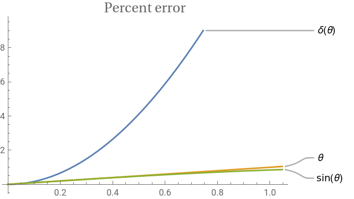
From the graphic, it is visible that θ and are similar in this interval with a small percentual error. Thus, it is expected that the behaviour of a “linear pendulum” is similar to that of a “sinusoidal pendulum”.
sin(θ)
0,
π
3
Creating the linear pendulum
Creating the linear pendulum
Analytical solution
Analytical solution
To create the pendulum, we first need to solve the differential equation to obtain the function modeling the angle between the rod and the vertical axis. We will obtain the solution for the linear equation by asigning specific values to different important parameters: first, we define , which is easily recognized as the acceleration due to gravity, hence we say is a good approximation.As for the rest of parameters, that is, the length of the rod, the starting angle, and the initial velocity, we will let them expressed by arbitrary names respectively.
g
g=9.81
m
2
s
L,α,ω
In[]:=
linearsol=DSolveValueθ''[t]+θ[t]==0,θ'[0]==ω,θ[0]==α,θ,t
9.81
L
Out[]=
Function{t},1.αCos+0.319275
3.13209t
L
L
ωSin3.13209t
L
We will now assume specific values for the parameters, let’s say and . With this, we can create the function for the angle given by time.
L=6,α=π/6
ω=0
In[]:=
linearθ[t_]=linearsol[t]/.{L->6,α->Pi/6,ω->0}
Out[]=
0.+0.523599Cos[1.27867t]
Plotting this expression for the first 20 seconds:
In[]:=
Plot[linearθ[t],{t,0,20},AxesLabel->{"Time(s)",θ},PlotStyle->Lighter[Pink]]
Out[]=
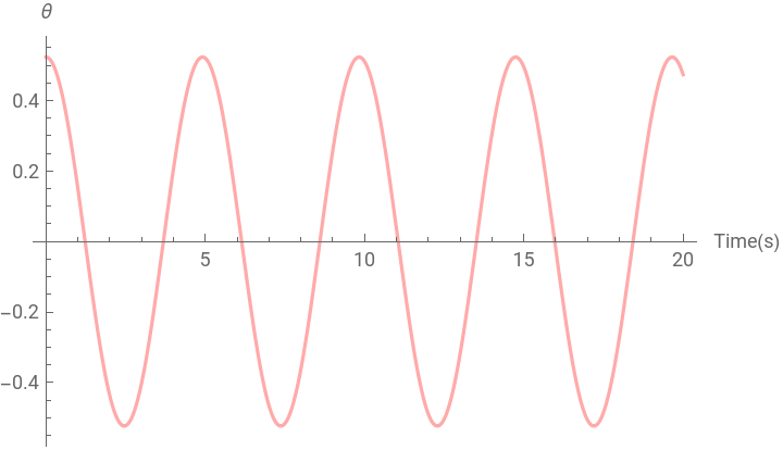
Notice that the maximum amplitude for the function does not change, this is expected as there are no external forces draining energy from the system.
Graphics
Graphics
We can now visualize all the elements from the system. I will start by creating the roof and the vertical axis from which the angle θ is measured.
In[]:=
roof=Graphics[{Brown,Thickness[0.01],Line[{{-5,0},{5,0}}]}];verticalaxis=Graphics[{Green,Dashed,Thickness[0.002],Line[{{0,10},{0,-10}}]}];Show[roof,verticalaxis,PlotRange->{{-5,5},{0,-10}}]
Out[]=
To properly get the pendulum (rod and mass), we will need to know its coordinates. Assuming the origin is at the intersection of the roof with the vertical axis, we notice (with a bit of trigonometry) that its coordinates are given by:
(0,0)
X
l
(
3
)Y
l
(
4
)Where is the length of the rod. With this, we can look at the position of the pendulum at .
L
t=0
In[]:=
linearX[t_]:=6*Sin[linearθ[t]]linearY[t_]:=-6*Cos[linearθ[t]]Print["Position of the mass at t=0: ","{",linearX[0],",",linearY[0],"}"]
Position of the mass at t=0: {3.,-5.19615}
To visualize it, we just need to create the mass, which I will show as a circle, and the rod will be shown as a line connecting the origin and the center of the mass.
In[]:=
linearpendulum[t_]=Graphics[{Blue,Thickness[0.003],Circle[{linearX[t],linearY[t]},0.35],Line[{{0,0},{linearX[t],linearY[t]}}]}];Show[roof,verticalaxis,linearpendulum[0],PlotRange->{{-5,5},{0,-10}}]
Out[]=
To see the full movement, we just need to animate this.
In[]:=
Animate[Show[roof,verticalaxis,linearpendulum[t],PlotRange->{{-5,5},{0,-10}}],{t,0,10},AnimationRate->2.5,SaveDefinitions->True]
Out[]=
Creating the sinusoidal pendulum
Creating the sinusoidal pendulum
Numerical solution
Numerical solution
Graphics
Graphics
And we create the graphic object of the pendulum:
Animating this result
Comparison
Comparison
Original problem
Original problem
Finally, with both solutions obtained, we can compare different things. I will start taking a look at the function obtained that models the angle θ. Plotting said function for both approaches at the same time:
As expected, the two solutions differ from each other. The linear approach seems to be having a slightly faster period which results in its plot being more horizontally compressed.
We can also animate both pendulums at the same time, making the difference more obvious to the eye:
We can also animate both pendulums at the same time, making the difference more obvious to the eye:
To see how much the result varies we can use the same technique of the percent error (assuming the numerical solution as the correct answer):
We see two important things: the first is that the maximum value of the error is increasing with each cycle of the pendulum, and that the range between the maximum and the minimum value is decreasing.
Changing the starting angle
Changing the starting angle
Pendulums as graphic objects
And finally animating both pendulums:
Acquiring the same plots from the previous version:
It is clear that the behaviour of the linear approximation is completely different from the sinusoidal function. This results in an error function with more chaotic spikes.
References
References
1
.Henry Edwards, Charles, E. Penney, David and Calvis, David. Differential Equations and Boundary Value Problems. 5th. s.l. : Pearson, 2019.