The stationary solutions of the Klein-Gordon equation refer to solutions that are time-independent, meaning they remain constant over time. For the non-linear Klein-Gordon equation you are discussing:
-κ(-2+)-β
2
d
x
n
d
2
t
x
n+1
x
n
x
n-1
2
ω
x
n
3
x
n
Stationary solutions arise when the time derivative term, , is zero, meaning the motion of the system does not change over time. This leads to a static differential equation:
2
d
x
n
d
2
t
-κ(-2+)-β
x
n+1
x
n
x
n-1
2
ω
x
n
3
x
n
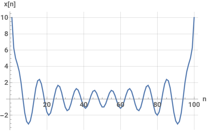
This equation describes how particles in the lattice interact with each other and how non-linearity affects the steady state of the system.
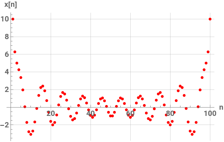
The solutions to this equation correspond to the various possible stable equilibrium states of the system, where each represents different static distribution patterns of displacements. The specific form of these stationary solutions depends on the system parameters, such as , , and , as well as the initial and boundary conditions of the problem.
To find these solutions in a more specific form, one might need to solve the equation using analytical or numerical methods, considering the different cases that could arise in such a non-linear system.
This equation describes how particles in the lattice interact with each other and how non-linearity affects the steady state of the system.
The solutions to this equation correspond to the various possible stable equilibrium states of the system, where each represents different static distribution patterns of displacements
x
n
κ
ω
β
To find these solutions in a more specific form, one might need to solve the equation using analytical or numerical methods, considering the different cases that could arise in such a non-linear system.
By interpreting the equation in this way, we can relate the dynamics described by the discrete Klein - Gordon equation to the behavior of DNA molecules within a biological system . This analogy allows us to understand the behavior of DNA in terms of concepts from physics and mathematical modeling .
In[]:=
numBases=100;(*Numberofbasepairs,representingasegmentofDNA*)kappa=1/10;(*Elasticityconstant,chosentoreflectthestiffness;arbitraryunit*)omegaD=2/10;(*Frequencyterm,speculativeandlowtoreflectslowdynamics*)beta=5/100;(*Nonlinearitycoefficientsmalltointroducemildnonlinearity*)(*Initializealistforthex_nvariables*)variables=Table[x[n],{n,1,numBases}];(*DefinetheequationsbasedonthediscretizedversionoftheKlein-Gordonequation*)equations=Table[-kappa(x[n+1]-2x[n]+x[n-1])==omegaD^2(x[n]-betax[n]^3),{n,2,numBases-1}];(*Addboundaryconditions,forexample,x[1]andx[numBases]fixedto0oranyothervalue*)boundaryConditions={x[1]==10,x[numBases]==10};(*Combinetheequationswiththeboundaryconditions*)fullSystem=Join[equations,boundaryConditions];(*Solvethesystemwithaninitialguessforeachvariable*)initialGuess=Table[{x[n],1/100},{n,1,numBases}];(*oranysmallvalueclosetoexpectedsolutions*)solution=FindRoot[fullSystem,initialGuess,Method->{"Newton","StepControl"->"TrustRegion"}];(*Extractthesolutionforplottingoranalysis*)solvedValues=Table[x[n]/.solution,{n,1,numBases}];(*Optionally,youcanplotthesolutiontovisualizethestationarystates*)ListPlot[solvedValues,PlotStyle->PointSize[Medium],Joined->True,GridLines->Automatic,PlotRange->All,AxesLabel->{"n","x[n]"},LabelStyle->{"Medium",Bold}]
Out[]=
In[]:=
ListPlot[solvedValues,PlotStyle->{Red,PointSize[Medium]},GridLines->Automatic,PlotRange->All,AxesLabel->{"n","x[n]"},LabelStyle->{"Medium",Bold}]
Out[]=
In[]:=
dataForPlot=Table[{n,0,solvedValues[[n]]},{n,1,Length[solvedValues]}];ListPointPlot3D[dataForPlot,PlotStyle->{Red,PointSize[Medium]},AxesLabel->{"n","Index","x[n]"}]
Out[]=

Example 1: Increased Elasticity Constant
Example 1: Increased Elasticity Constant
In[]:=
Clear["Global`*"];
In[]:=
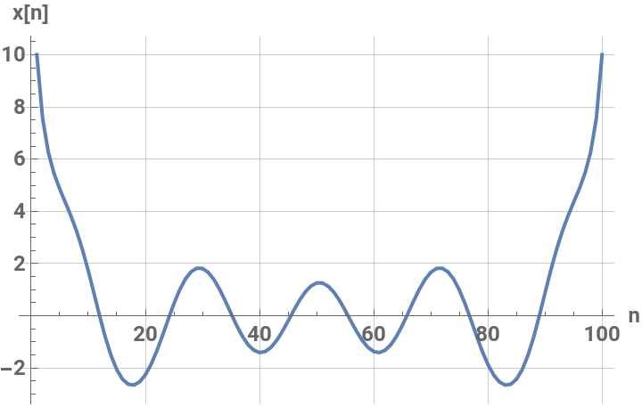
numBases=100;kappa=5/10;(*Increasedelasticityconstant*)omegaD=2/10;beta=5/100;variables=Table[x[n],{n,1,numBases}];equations=Table[-kappa(x[n+1]-2x[n]+x[n-1])==omegaD^2(x[n]-betax[n]^3),{n,2,numBases-1}];boundaryConditions={x[1]==10,x[numBases]==10};fullSystem=Join[equations,boundaryConditions];initialGuess=Table[{x[n],1/100},{n,1,numBases}];solutionIncreasedKappa=FindRoot[fullSystem,initialGuess,Method->{"Newton","StepControl"->"TrustRegion"}];solvedValuesIncreasedKappa=Table[x[n]/.solutionIncreasedKappa,{n,1,numBases}];ListPlot[solvedValuesIncreasedKappa,PlotStyle->PointSize[Medium],Joined->True,GridLines->Automatic,PlotRange->All,AxesLabel->{"n","x[n]"},LabelStyle->{"Medium",Bold}]
Out[]=
In[]:=
ListPlot[solvedValuesIncreasedKappa,PlotStyle->{Red,PointSize[Medium]},GridLines->Automatic,PlotRange->All,AxesLabel->{"n","x[n]"},LabelStyle->{"Medium",Bold}]
Out[]=
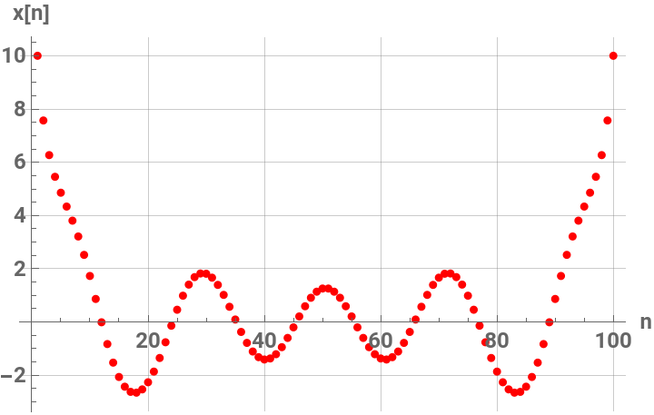
In this example, the elasticity constant is increased to 0.5, representing a system with greater stiffness . This parameter influences how resistant the system is to deformation, implying that a higher makes the system more resilient to changes . By increasing , we are essentially tightening the interactions between adjacent units in the model, which could represent, for instance, stronger bonding forces in a physical or biological system .
κ
κ
κ
Example 2: Increased Nonlinearity Coefficient
Example 2: Increased Nonlinearity Coefficient
Refferences
Refferences
1
.Frantzeskakis, D. J., Karachalios, N. I., Kevrekidis, P. G., Koukouloyannis, V., & Vetas, K. (2019). Dynamical transitions between equilibria in a dissipative Klein–Gordon lattice. Journal of Mathematical Analysis and Applications, 472(1), 546-576.
2
.Englander, S. W., Kallenbach, N. R., Heeger, A. J., Krumhansl, J. A., & Litwin, S. (1980). Nature of the open state in long polynucleotide double helices: possibility of soliton excitations. Proceedings of the National Academy of Sciences, 77(12), 7222-7226.