Deep learning is becoming commonplace in many fields of science and technology. The ability to identify and predict patterns in large data sets is a powerful tool, and can in fact, replace many brute-force and calculation/simulation intensive methods. Traditionally, identifying molecular vibrational modes, and hence the corresponding IR-spectra for organic molecules is a non-trivial process.Theoretically, it is performed by specialized ab initio quantum chemistry software, and is a time-consuming process. Experimentally, it is determined by specialized spectrometers. This project is aimed at predicting such inherent patterns between parametrized molecular physical/chemical properties, and their vibrational modes.
Here, we focus on two major aspects. First, we introduce a method to write, execute and animate input and data files to a third party quantum chemistry software (Orca) through the Wolfram Language (WL). Next we use this freshly generated vibrational spectra data to try and predict patterns using a variety of machine learning functionalities.
Here, we focus on two major aspects. First, we introduce a method to write, execute and animate input and data files to a third party quantum chemistry software (Orca) through the Wolfram Language (WL). Next we use this freshly generated vibrational spectra data to try and predict patterns using a variety of machine learning functionalities.
Introduction
Introduction
An infrared or vibrational spectrometer is an instrument that experimental chemists, materials scientists and other researchers use to identify or “characterize” chemical substances. When the molecules of an unknown chemical substance are made to interact with infrared radiation, the molecules absorb the radiation, shift to an excited state, and dissipate energy in the form of molecular vibrations. These vibrations are either symmetric or antisymmetric, giving rise to many sub-varieties (stretching, scissoring, rocking, wagging, twisting, out-of-plane). While the near-IR is responsible for molecular vibrations, the far-IR corresponds to more rotation dominant behavior.
In[]:=
Style/@Text/@TextSentences[WikipediaData["Infrared spectroscopy"]][[;;3]]//Column
Out[]=
Infrared spectroscopy (IR spectroscopy or vibrational spectroscopy) involves the interaction of infrared radiation with matter. |
It covers a range of techniques, mostly based on absorption spectroscopy. |
As with all spectroscopic techniques, it can be used to identify and study chemical substances. |
Now, the question is, given enough descriptor parameters for a molecule, or as it is commonly known as a "molecular fingerprint" (discussed further below), can we predict the vibrational modes that it would exhibit? Vibrations are the result of chemical bonds executing harmonic oscillations, and are highly specific to the type of atoms involved in the bond, and the overall structural and energy landscape. However, they are also not trivial, and are commonly calculated using quantum chemistry software that rely on Density Functional Theory (DFT) principles such as the Born - Oppenheimer (BO) approximations, among others. Hence, this is a perfect example of hard-to-compute data with a rich set of identifiable patterns. This project deals with the generation of such data, and the construction of neural network models to best predict vibrational modes, given a unique molecule.
This is what an IR spectra plot for an organic molecule “aniline” looks like. The frequency, commonly measured in wavenumber (1/cm), has a corresponding value of transmittance.
In[]:=
WebImageSearch["Infrared spectroscopy"];
In[]:=
%[[3]]//Magnify[#,0.75]&
Out[]=
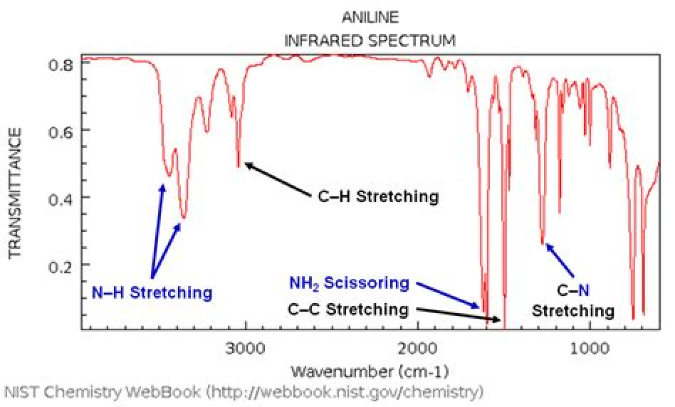
The lower the transmittance, the greater the absorption and hence the vibrational mode. Thus, we can characterize the “most significant” frequencies as the ones with the lowest transmittance values.
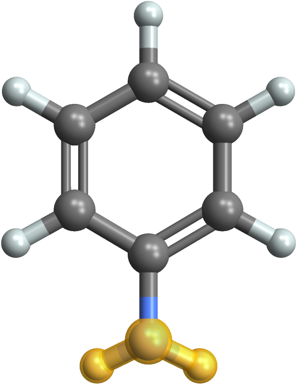
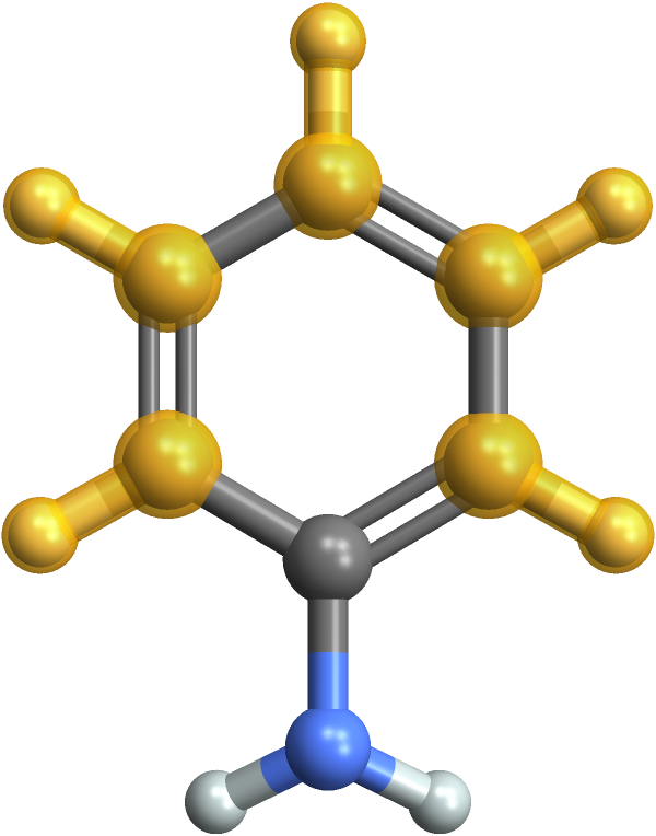
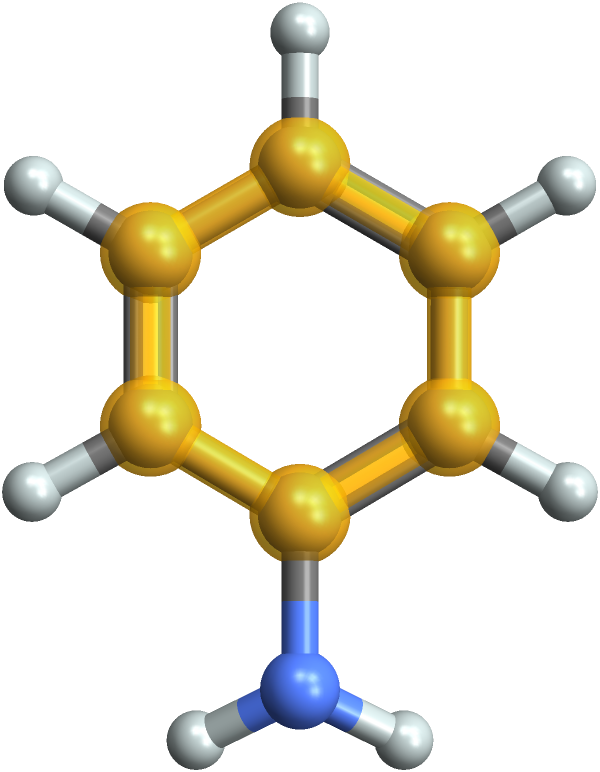
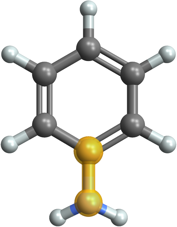
Highlighted in yellow are the bonds that exhibit the various stretching modes as shown above for aniline, in decreasing order of frequency:
In[]:=
Function[bond,{Image@MoleculePlot3D[Molecule@"Aniline",{Bond[First@bond,"Single"|"Aromatic"]}],Style[Text@bond/.{{a_,b_},c_}a<>"-"<>b<>" "<>c,FontSize20]}]/@{{{"N","H"},"~3400 "},{{"C","H"},"~3000 "},{{"C","C"},"~1500 "},{{"C","N"},"~1300 "}}//Transpose//Grid[#,FrameAll]&
-1
cm
-1
cm
-1
cm
-1
cm
Out[]=
N-H ~3400 -1 cm | C-H ~3000 -1 cm | C-C ~1500 -1 cm | C-N ~1300 -1 cm |
Even molecules have fingerprints~
Even molecules have fingerprints~
We can identify each molecule with a unique fingerprint in the form of the “radial distribution function”(RDF), a model that describes the variation of atom density as a function of distance from a reference atom:
In[]:=
WebImageSearch[SearchQueryString@"Radial distribution function dr"][[{4,7}]]//ImageCollage[#,Automatic,400]&
Out[]=
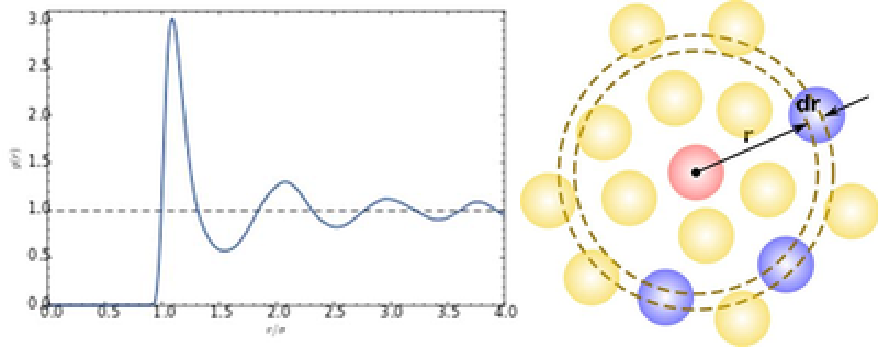
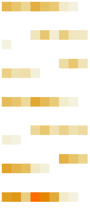
RDF values in the WL are a set of discrete values in a {210} numeric array, which is based a list of molecular descriptors calculated by Dragon[1, 2]
In[]:=
Molecule[#]["RDF"]&/@{"ethanol","acetic acid","acetone"}
Out[]=
NumericArray,NumericArray,NumericArray

Although the differences seem subtle, they are based on highly sensitive parameters.
In[]:=
MatrixPlot[Partition[Normal@#,9],FrameFalse]&/@%//Grid[{#,{"ethanol","acetic acid","acetone"}},FrameAll]&
Out[]=
ethanol | acetic acid | acetone |
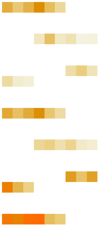
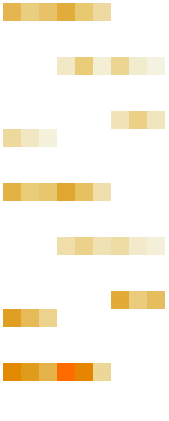
The RDF in the WL has 7 crucial parts (1 unweighted and 6 weighted) that make it ideal for fingerprinting and “deploy-worthy” in NNs:
1
.Pure radial distribution parameter
2
.Molecular mass
3
.Van der Waals volume
4
.Sanderson electronegativity
5
.Polarizability
6
.Ionization potential
7
.I-state (intrinsic-state from local vertex variants)
Data sets- Let’s automate things!
Data sets- Let’s automate things!
Now, we need to find a suitable software that will generate our dataset for us. Among a wide range of software that can do this, I found Orca[3] to be the most suitable. It has a very simple installation procedure, and is windows-compatible. An easy to follow documentation is a huge plus.
In[]:=
Style/@Text/@TextSentences[WikipediaData["ORCA (quantum chemistry program)"]][[;;2]]//Column
Out[]=
"ORCA is an ab initio quantum chemistry program package that contains modern electronic structure methods including density functional theory, many-body perturbation, coupled cluster, multireference methods, and semi-empirical quantum chemistry methods." |
"Its main field of application is larger molecules, transition metal complexes, and their spectroscopic properties." |
An exciting bonus here is that not only can Orca generate data sets to do IR spectra (vibrational; absorption) analysis, but it can also be extended to study and predict patterns in Raman (vibrational; scattering), UV-vis (electro-optical), and NMR (magnetic) spectra.
General notes:
1
.Computation time: ~15 min for 20 atom system [geometry optimization + spectra calculations]
2
.Command line run software
From molecule name to spectra, all on our dear Mathematica
From molecule name to spectra, all on our dear Mathematica
We will perform execution and acquisition of data from Orca all through the WL. This will help internalize our entire process of data set generation. Orca requires 2 types of files to calculate the Hessian values for various organic molecules. They are the input and the data files. The data file is fairly straightforward; using the built-in function Molecule[], we can export .xyz data. The input file is very short and describes the method of energy minimization etc. which can be written as a string expression in the WL. First we download the software.
From here, code can be run only if Orca and its executable files are installed at "C:\\ Orca" from the link above.
(*CreateDirectory[FileNameJoin[{NotebookDirectory,"orca data"}]]*)
We can acquire ordered molecule name lists from the “GDB-9” database. We will leave it uncompressed until necessary, to save time.
In[]:=
dataGDB=CloudGet@CloudObject["https://www.wolframcloud.com/obj/jasonb/Compressed_GDB-9_molecules"];
Next, we shall consider smaller molecules (<=20 atom systems) so that the computation time does not overflow, while at the same time ensuring that we still have a diverse representation of functional groups (and hence a diverse representation of vibrational frequencies). Additionally, some uncommon molecules do not have IUPAC name in the PubChem service, and hence those are removed.
newMoldata[n_,m_]:={#,Molecule@#}&/@Last/@First/@(Select[(ServiceExecute["PubChem","CompoundProperties",{"Molecule"#,"Property"{"IUPACName"}}]&/@Select[Uncompress/@dataGDB[[n;;m]],BondCount@#≤20&]),!StringContainsQ[ToString@FullForm@#[[1]],"Missing"]&])
Each time we wish to add data for new molecules, we take a part of the GDB database in serial order (serial 81 through 120 in this example, meaning the first 80 have been completed and saved in the “orca data” folder in the NotebookDirectory):
In[]:=
new=newMoldata[121,140];
As the quantum chemistry simulations are time-consuming, we should perform a sanity check to see if some molecules have already been computed, then define a list of fresh molecules to compute:
In[]:=
currentMoldata={#,Molecule@#}&/@StringReplace[(ToLowerCase/@StringCases[#,"data"~~_~~x__~~"_out_"->x]&/@FileNames[___~~"_out_IR.txt",FileNameJoin[{NotebookDirectory[],"orca data"}]]//Flatten),StartOfString~~"n-""N-"];
A visual check if we have diversity in the types of organic bonds:
List of molecules to compute (example run):
And here we automate the process:
Our Data are on Cloud (nine)
Our Data are on Cloud (nine)
We will need to access this data often. It will be saved in the form:
However, this data is not ready yet. We need to do some cleaning, and make it variable by choice by introducing a parameter:
1
.Some peaks are very insignificant and can be discarded (very high relative transmittance values)
2
.Some values fall outside the usual IR frequency range of 400-4000 cm-1, we can specify a new range to restrict our search
3
.Finally, some peaks are extremely close, separated by <10 cm-1. A parameter is used to set that frequency width and return the most prominent peak within it
4
.The molecules are also in name order, better to RandomSample to be safe.
Alternatively, it can be exported as a “.mx”:
So you have the numbers, but can you animate it?
So you have the numbers, but can you animate it?
Numbers are hard to understand, let us try to animate these molecular vibrations.
And here it goes :
Let's try this for a random molecule :
Now we have the data and coordinate points! We need to specify the frame rates and adjust the animation so it can run smoothly [5]
There are quite a few vibrational modes for this molecule ~20, so we will just animate 3 random ones. These vibrations are highly accurate as they retain all trajectory data that were calculated :
Predicting frequencies using self normalizing neural nets (SNNs)
Predicting frequencies using self normalizing neural nets (SNNs)
NNs are nit - picky towards data format
NNs are nit - picky towards data format
First, we try to work on this problem statement- Given a trained molecule (and hence its RDF), and an arbitrary transmission intensity, can we assign the intensity value to a suitable vibrational frequency?
We include copies of random variate data for each molecule to account for variability in intensity
We split the dataset twice, such that we have “forTrain” which accounts for a “traininset” and a “validationset”, and we have “forTest” which is exclusively kept for testing new molecules.
SNN time!
SNN time!
We will use a self-normalizing NN:
Standardize our data:
Clearly, the minimization of loss is not very efficient, let us test this-
These pairs are the correct output options for {frequency, intensity}
Now to visualize the results of our final test, we can plot a histogram of counts versus the absolute difference between predicted values and actual values of frequencies.
Ideally, we would want to have-
1) Maximum number of counts in the 0-200 cm^-1 range; we need an early sharp peak
2) Very narrow range of distribution, terminating at ~500-600 cm^-1
1) Maximum number of counts in the 0-200 cm^-1 range; we need an early sharp peak
2) Very narrow range of distribution, terminating at ~500-600 cm^-1
This requires further tweaking of SNN parameters and perhaps restructuring the datasets. Among other things, we have also tried a seq-to-seq recurrent neural network (see full notebook) before moving on to the SNN. Unfortunately, it was not very successful. This points us to the future direction of this work. Fundamentally, this kind of exploration is quite new, and while reports exist in the literature, they are highly restricted to analyzing 1-2 molecules per study, and after thorough training[5].
What did we just do?
What did we just do?
◼
We have shown without doubt that the Wolfram Language can be used to interface, write scripts and run third-party software with ease. This can be extended to other software that lack a UI, or are tedious to set up.
◼
We have generated a large data set of organic molecules and their vibrational modes (>100 molecules). This is handy data for those who wish to skip the ab initio calculations altogether.
◼
We have animated these vibrational modes on the WL to create visually informative GIFs
◼
We have explored Classifiers, SNNs and RNNs towards predicting IR spectra information
Where do we go from here?
Where do we go from here?
So, we finally come to the end of the WSS2020.
But does the exploration stop here? Not in the slightest!
We did a lot along the way, but we still have the larger picture to work towards.
But what are our options? Working with ideas, we have a few paths we can take-
But does the exploration stop here? Not in the slightest!
We did a lot along the way, but we still have the larger picture to work towards.
But what are our options? Working with ideas, we have a few paths we can take-
◼
Certainly, we start with tweaking the current SNN, modifying the architecture and dataset format to make it more conducive to find patterns.
◼
Due to the uniqueness of our data format, multi-target regression neural networks seem to be a good approach. This would include an additional part in the network that would account for deciding if and when a new "frequency-intensity" pair needs to be added to the output depending on the input RDF.
◼
Another possible route is to convert our data into images and work from there; the RDF would be represented as an ArrayPlot for example, or even just as the MoleculePlot, and the output freq-intensity would take the form of coordinate dots on a 2D plot. This will solve a few problems and give rise to new ones, but it is certainly worth a try.
◼
A third and interesting route is to use WaveNet, as the RDF has periodic patterns similar to that of acoustic waves. This method would leverage on the RDF periodicity to tag frequency to transmittance.
Keywords
Keywords
◼
Infra-red/ vibrational spectra
◼
radial distribution function
◼
molecular fingerprints
◼
regression neural networks
◼
self-normalizing neural networks
Acknowledgment
Acknowledgment
Mentor: Tuseeta Banerjee
The Summer School was a unique experience for me. It has pushed me beyond what I thought I could do in such a short period, especially working remotely across a wide time zone gap and during an ongoing pandemic. Despite a few personal emergencies that put a delay on my work, the whole WSS2020 team- all the staff, mentors, and students, have been extremely supportive and understanding. When I joined the school, I wished to become more “fluidic, natural and intuitive” in my way of coding in the Wolfram Language, and through the many exercises, problems and of course, the project, I am certain that I have taken a huge step towards this goal. Above all- I wanted to learn as much as possible, to help and be helped, and to make many friends along the way, and I have absolutely no doubts that I have achieved this. Lastly, and most importantly, I give my sincerest thanks to Tuseeta, whom I would like to call my mentor as well as my friend. In a nutshell, the WSS2020 has been everything I wished it would be, and while the school comes to an end, the project will continue, and so will the learning.
References
References
1
.Puzyn, T., Leszczyński, J. & Cronin, M. Recent Advances in QSAR Studies: Methods and Applications. Springer (2010).
2
.List of molecular descriptors calculated by Dragon. 1–51 http://www.talete.mi.it/products/dragon_molecular_descriptor_list.pdf.
5
.Kananenka, A. A., Yao, K., Corcelli, S. A. & Skinner, J. L. Machine Learning for Vibrational Spectroscopic Maps. J. Chem. Theory Comput. 15, 6850–6858 (2019).