Problem
Problem
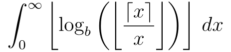
Given b is greater than 1, find the value of the following integral
Out[]=
Visualization
Visualization
Michael Penn discussed this eccentric integration from CRUX on this channel recently. Please use the link to watch the video. The main idea is to show that, given b > 1, the integrand is zero when x is no less than 1. For x is strictly between 0 and 1, the integrand is a piecewise function with different constant value on infinite number of partitions such as , ) for k in integer domain. Eventually the final result comes down to summing up a geometric series.
(1/
k
b
1/
k+1
b
I feel LogLinearPlot helps to visualize the problem in a straightforward manner. For convenience, I can let b = , the base of nature logarithm and take a look at the case with finite terms. For instance, I pick up 16 terms
In[]:=
nTerms=16;
In[]:=
range=Range[nTerms]
Out[]=
{1,2,3,4,5,6,7,8,9,10,11,12,13,14,15,16}
The key to proper visualization is to set proper ticks to represent the switching positions. In Ticks option, I can add symbolic logarithm base to the x axis
In[]:=
xTicks=With[{val=^(-range),label=Power[b,HoldForm[-#]]&/@range},Transpose[{val,label}]];
In[]:=
yTicks=range;
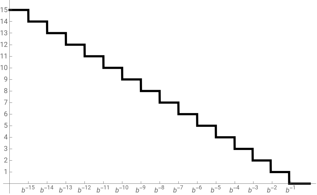
If I plot the integrand with LogLinearPlot, the interesting pattern of ascending stair (right to left) definitely gives away the hidden secret of the problem.
In[]:=
plot=LogLinearPlot[Floor[Log[Floor[Ceiling[x]/x]]],{x,^-nTerms,1},PlotStyle{Black,Thickness[.007]},ExclusionsNone,Ticks{xTicks,yTicks},TicksStyleDirective["Label",11]]
Out[]=
In Michael’s video he mentioned there are two ways to do the integral and I use two different color stripe systems to show them. The first one is just sum up the area of the vertical color stripes. Notice that if any graphics object is added to LogLinearPlot, the x coordinate must be the value of the input. Say, I want to add a point at ,2), the actual coordinate used in Epilog-like option is (-3,2)
log
b
(
-3
b
In[]:=
nthVerticalRect[n_]:=Rectangle[{-n-1,0},{-n,n-0.05}]
In[]:=
Show[plot,PlotStyleRed,Epilog{Opacity[0.6],{Hue[#/nTerms],nthVerticalRect[#]}&/@Most[range]}]
Out[]=
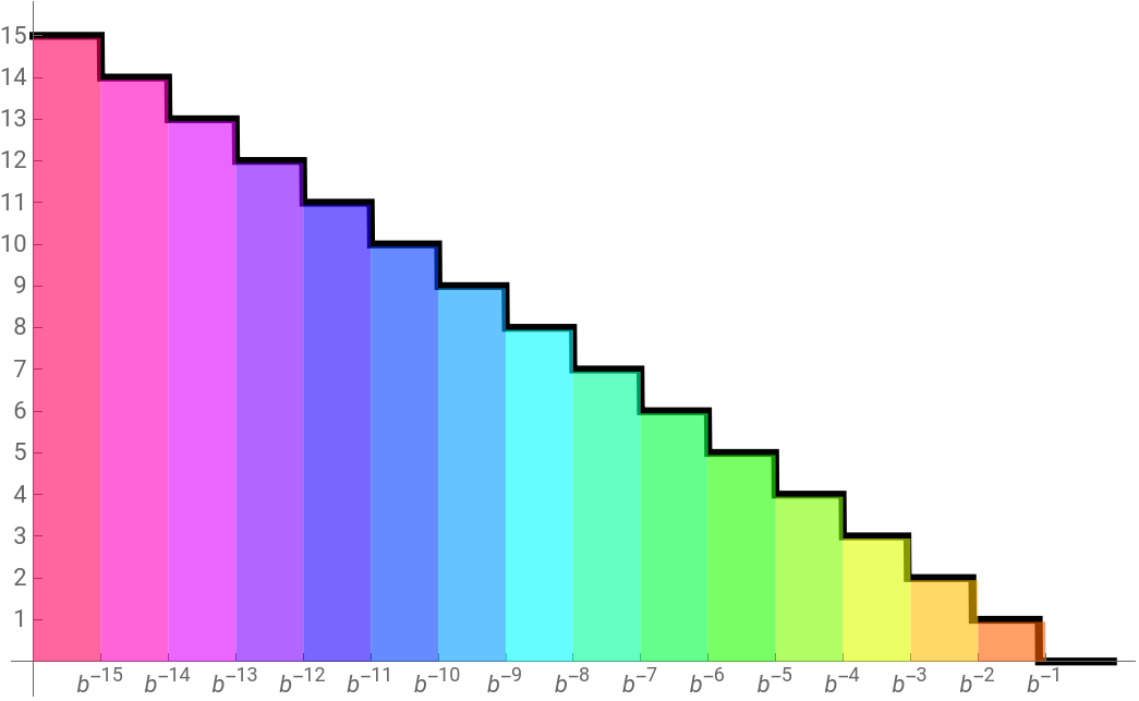
Because the area of each stripe is width times height, the infinite integral is just the sum of all vertical stripes. Warning: the color stripes are NOT of constant width, if they are plotted on linear scale for x axis, the widths are squeezed at exponential speed as it goes from 1 to 0
In[]:=
res1=Sumn*-,{n,1,Infinity},Assumptionsb>1
1
b^n
1
b^(n+1)
Out[]=
1
-1+b
The second way is to flip the color stripe and I can sum of the area of horizontal ones.
In[]:=
nthHorizontalRect[n_]:=Rectangle[{-nTerms,n-1},{-n-0.05,n}]
In[]:=
Show[plot,Epilog{Opacity[0.6],{Hue[#/nTerms],nthHorizontalRect[#]}&/@Most[range]}]
Out[]=
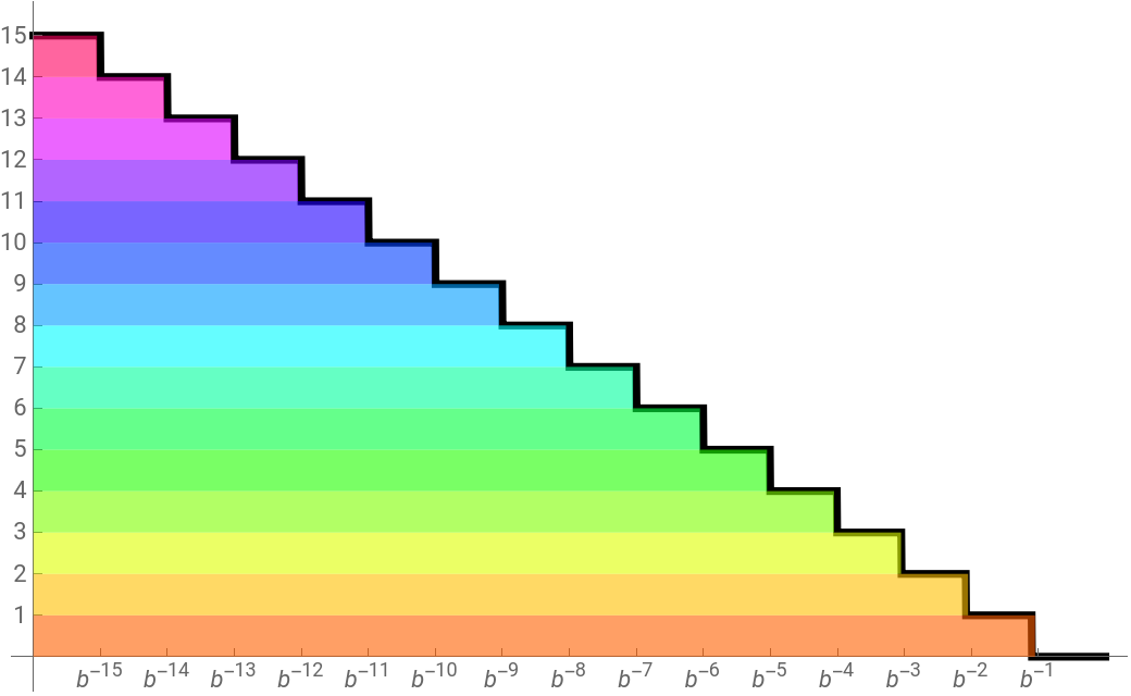
This way I have a simpler expression for area sum because of the constant height of each color stripe and each width is a term of geometric series, thus the integral is
In[]:=
res2=Sum,{n,1,Infinity},Assumptionsb>1
1
b^n
Out[]=
1
-1+b
Verify two results are the same
In[]:=
res1res2
Out[]=
True
Summary
Summary
◼
LogLinearPlot is useful to visualize geometric series
◼
Ticks in LogLinearPlot can be set along with customizable labels
◼
Using graphics object in log plot needs coordinate conversion