Daily financial data in the form of {open, high, low, close, volume}, prices and volume, have been available to investors to summarize market data for about a century. This notebook is an experiment to see if the Mathematica machine-learning Predict function can predict a 21 day forward price, using a numerical tensor containing the previous quarter of {date, open, high, low, close, volume} data. The input length of a quarter is chosen to include volatility around earnings reporting in each training set. The data collected by FinancialData are stored in a Dataset, which is converted to a numerical tensor using a few different preprocessing strategies.
Data set
Data set
This notebook is designed so that sym can be changed to any symbol available in FinancialData, then the whole notebook can be evaluated using the new symbol. Data collection is started in 2002 to avoid the missing week of data in September 2001.
In[]:=
sym="SPY";data0={#1,QuantityMagnitude[#2]}&@@@Normal[FinancialData[sym,"OHLCV",{2002}]];
In[]:=
keys={"date","open","high","low","close","volume"};rsq=ConstantArray[0,5];(*usedtocollectRSquaredinformation*)
In[]:=
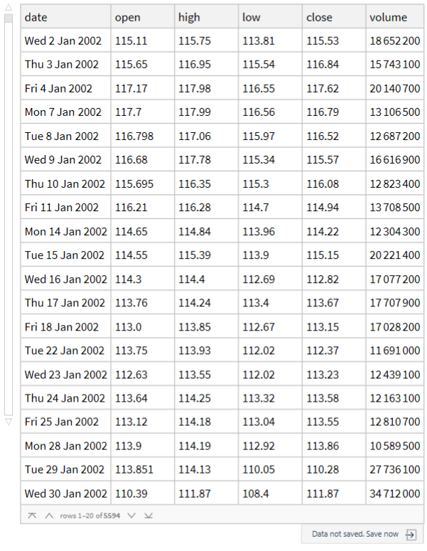
priceDS=AssociationThread[keys,#]&/@({DateObject[#1,"Day"],#2,#3,#4,#5,#6}&@@@(Flatten/@data0))//Dataset
Forward date from last date in data set.
In[]:=
DateRange[priceDS[[-1]][[1]],DatePlus[Today,{2,"Month"}],"BusinessDay",HolidayCalendar->{"UnitedStates","NYSE"}][[22]]
Out[]=
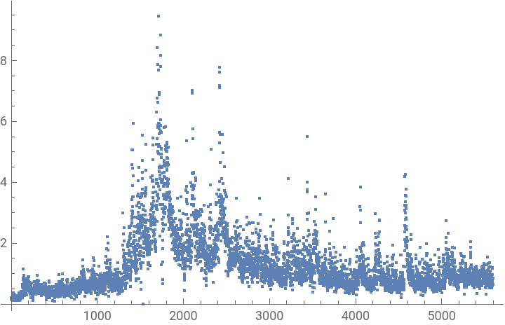
“volume” in the Dataset is represented as an integer, voladj is used to scale by the geometric mean to get a smaller Real input.
In[]:=
voladj=priceDS[GeometricMean[N@Select[#,#>0&]]&,"volume"]priceDS[ListPlot[#/voladj,PlotRange->All]&,"volume"]
Out[]=
9.21926×
7
10
Out[]=
Predict 1
Predict 1
This input strategy use all the financial data as usually reported converted to a numerical tensor. The date is in years starting at year 2000, in order to have smaller valued input.
In[]:=
set1=Normal@priceDS[All,<|"dateyear"->DateValue[#date,"YearExact"]-2000,"open"->#open,"high"->#high,"low"->#low,"close"->#close,"volume"->#volume/voladj|>&];
In[]:=
spoints=RandomInteger[{1,Length[set1]-84},1000];predictSet1=Values[Take[set1,{#,#+62}]]->set1[[#+84]]["close"]&/@spoints;
In[]:=
predict1=Predict[predictSet1,PerformanceGoal->"Quality",Method->"NearestNeighbors"]
Out[]=
PredictorFunction


In[]:=
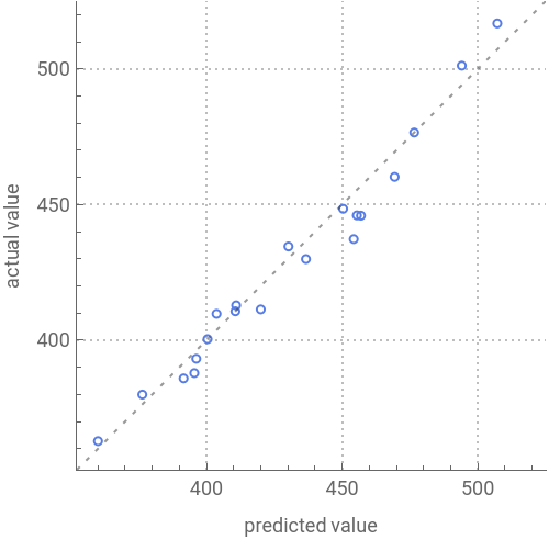
recentSet=Values[Take[set1,{#,#+62}]]->set1[[#+84]]["close"]&/@Take[Last/@Partition[Drop[Range[Length[set1]],-84],63,21],{-20,-1}];rsq[[1]]=PredictorMeasurements[predict1,recentSet,"RSquared"]PredictorMeasurements[predict1,recentSet]
Out[]=
0.966691
Out[]=

Predict 2
Predict 2
This strategy converts the {high low}, sequence, to a geometric mean of {high, low}, since the raw data always has the high before the low even though the prices may not have occurred in that order. This reduces the number of input prices each day to three.
In[]:=
set2=Normal@priceDS[All,<|"dateyear"->DateValue[#date,"YearExact"]-2000,"open"->#open,"geomean"->Sqrt[#high#low],"close"->#close,"volume"->#volume/voladj|>&];
In[]:=
spoints=RandomInteger[{1,Length[set2]-84},1000];predictSet2=Values[Take[set2,{#,#+62}]]->set2[[#+84]]["close"]&/@spoints;
In[]:=
predict2=Predict[predictSet2,PerformanceGoal->"Quality",Method->"NearestNeighbors"]
Out[]=
PredictorFunction
In[]:=
recentSet=Values[Take[set2,{#,#+62}]]->set2[[#+84]]["close"]&/@Take[Last/@Partition[Drop[Range[Length[set2]],-84],63,21],{-20,-1}];rsq[[2]]=PredictorMeasurements[predict2,recentSet,"RSquared"]PredictorMeasurements[predict2,recentSet]
Out[]=
0.964528
Out[]=
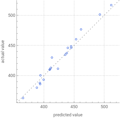
RSquared results for first two strategies.
Predict 3
Predict 3
This strategy changes the order of the {high, low} inputs to match the {open, close} trend. The actual data may not have occurred in this order but the strategy creates a day trend bias in the input.
Predict 4
Predict 4
This input strategy uses the same trend strategy as Predict 3, but changes all the price inputs to Log[price] to linearize potential exponential growth.
Predict 5
Predict 5
This strategy uses the FractalDC, fractal data compression, algorithm to reduce the size of the input excluding some of the less extreme inputs while preserving the first and last vectors. This has the effect of removing smaller day to day price changes in the close price. The algorithm has been previously presented Fractal market analysis. Predict 5 uses the same training sample as Predict 4 so the only difference between the two strategies is a compressed training and testing input. The first and last vectors of each input are the same.
FractalDC Code
The lengths of the training matrices are much shorter after the FractalDC processing.
RSquared for each method.
Model Projections with Current Data
Model Projections with Current Data
Graphic predictions are presented for a 21 trading day forward price from the last price in the data. The input data shows the variation of the daily price inputs and the projection to the forward price is a straight line. The x-axis is in decimal years since 2000, and the y-axis is price.
Time Series Forecast
Time Series Forecast
TimeSeriesForecast cannot handle a complicated input so the {DateObject, “close”} data are used for input.
Discussion
Discussion
This notebook was built up gradually and options and preprocessing strategies were adjusted based on testing. The Method “NearestNeighbors” seemed to get higher RSquared results on testing, so it was used in all the strategies. The “NeuralNetwork” method takes a lot of time and did not seem to get better results. The volume column was added last and doesn’t seem to improve the results, but I haven’t tested this carefully, intuitively it may be better input only price data without a method to specify that volume should be used for weighting. The input samples are blocks generated from a random starting point, if a particular Predict run tests with an RSquared less than 0.9, it is worth rerunning it to try a different training sample. I was surprised that the RSquared results could be so high; the Predictor Measurements have inputs biased toward more recent data. The whole thing needs to be prospectively tested.
There is enough variation of output that the algorithms will not likely be useful for long term trading, but the whole notebook could be changed to a shorter forward period and it could also be applied to minute data. This version may prove to be useful to predict market trends, but it will need a lot of testing. The Predict 5 strategy basically over-weights the tails of the input vectors so it should product more extreme forecasts even though it may have a high RSquared.
At this point I don’t know enough about neural networks to implement better input formats. The current results do seem to suggest that the 63 day input tensor may contain useful information.
CITE THIS NOTEBOOK
CITE THIS NOTEBOOK
Price prediction using a financial data tensor for training
by Robert Rimmer
Wolfram Community, STAFF PICKS, March 25, 2024
https://community.wolfram.com/groups/-/m/t/3147066
by Robert Rimmer
Wolfram Community, STAFF PICKS, March 25, 2024
https://community.wolfram.com/groups/-/m/t/3147066