The number of satellites being launched into orbit has dramatically increased in recent years. To address this problem we have developed a mathematical method for estimating the probability of collisions between pairs of satellites. As there are a large number of potential collision events, it becomes a computationally hard problem to sort through all such satellite collision pairs. Utilizing ergodic theory and discrepancy theory, we reduce this computationally hard problem into a simple evaluation of volume integrals. In this essay we provide a brief overview and illustrations of the main ideas underlying this approach.
The Kessler Effect
The Kessler Effect
A Brief History
A Brief History
In 1957 the space age began. The world’s first satellite - the Sputnik - was launched into space. It became a strategic necessity to maintain situational awareness of orbital objects. In quick succession NORAD (US North American Space Command) was founded, whose mission it was to curate a database of any satellites position and orbital characteristics with TLE’s (Two Line Elements).
We have the TLEs of the ISS (International Space Station):
ISS (ZARYA) 1 25544U 98067A 26197.86314870 .00003748 00000+0 76099-4 0 99982 25544 51.6311 153.2312 0006736 304.1301 55.9047 15.49027546576359
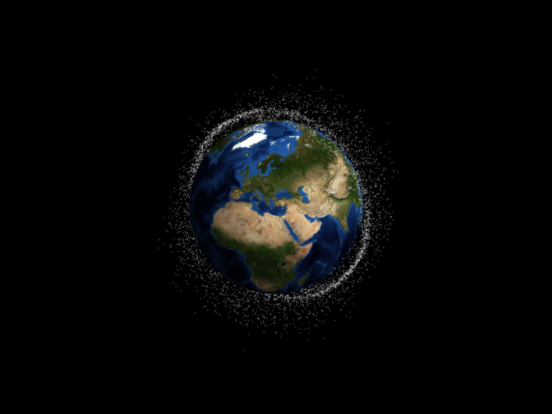
Around 20 years later, in 1978, the “Kessler effect” named after NASA scientist Donald J. Kessler was coined in a famous Popular Science article. This is a hypothetical phenomenon whereby in highly dense orbital regions around the earth, a runaway chain reaction of satellite collisions and resulting debris collisions occurs. Soon after in 1979, the NASA Orbital Debris program was founded to monitor and help mitigate the amount of debris orbiting the earth.
Orbital debris depiction around the earth:
How about now?
How about now?
The annual number of objects being launched into space has massively increased in the past 10 years from around 200 objects to over 4,500 objects. Multiple times on a daily basis, satellites pass within only a few kilometres of each other. As there is a large number of potential collision events, it becomes a hard problem to sort through all satellite collision pairs. Estimating satellite collision risk live is difficult, as getting precise and up-to-date satellite position data is not always possible. A central goal of this project is to make this hard problem tractable.
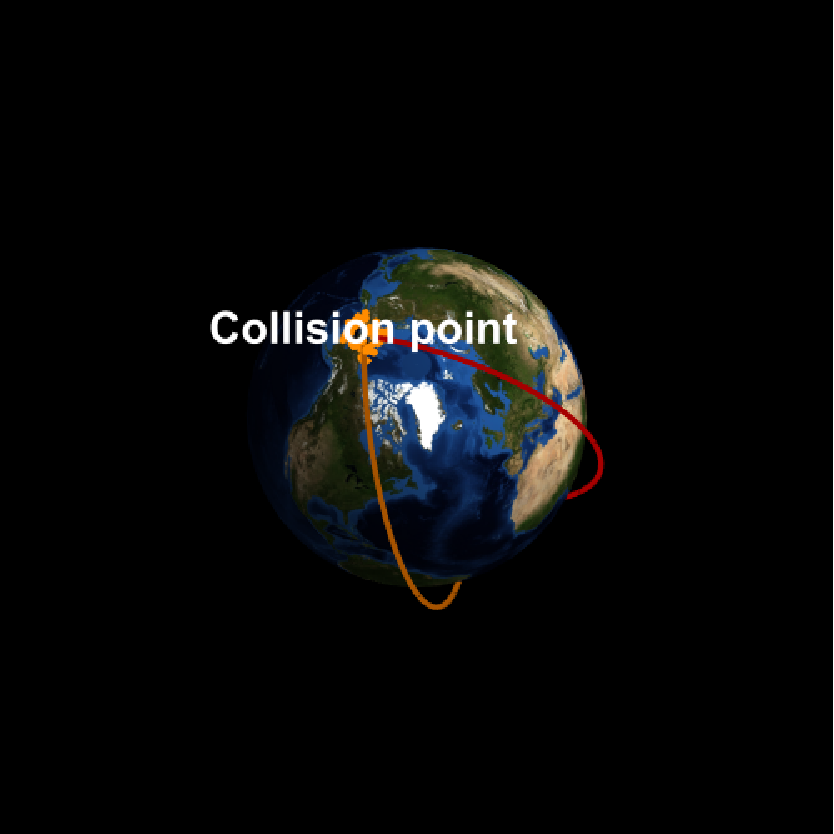
We will illustrate the 2009 satellite collision between an active Russian Iridium 33 and a defunct Kosmos 2251 satellite, as a real-world example of how small errors can lead to catastrophic failure. The predictions obtained using CELESTRAK data expected these satellites to miss each other by around 1/2 kilometres.
We will illustrate the 2009 satellite collision between an active Russian Iridium 33 and a defunct Kosmos 2251 satellite, as a real-world example of how small errors can lead to catastrophic failure. The predictions obtained using CELESTRAK data expected these satellites to miss each other by around 1/2 kilometres.
Plot of 2009 collision between a Russian Iridium 33 and a Kosmos 2251 satellite:
As of now, there is no international law for mandatory disposal of defunct satellites, although countries individually have regulations in place for decommissioning satellites. For example, the United States has a regulation in place requiring satellites to be deorbited within a 25 year time window. Unfortunately, there is little regulation implemented in practice though. Additionally, there are also concerns with regards to future satellite collision resulting from a large increase in the number of satellites being launched into orbit each year, many of which are contributed by large scale satellite constellations, such as SpaceX Starlink.
Kepler’s First Law
Kepler’s First Law
Why it fails?
Why it fails?
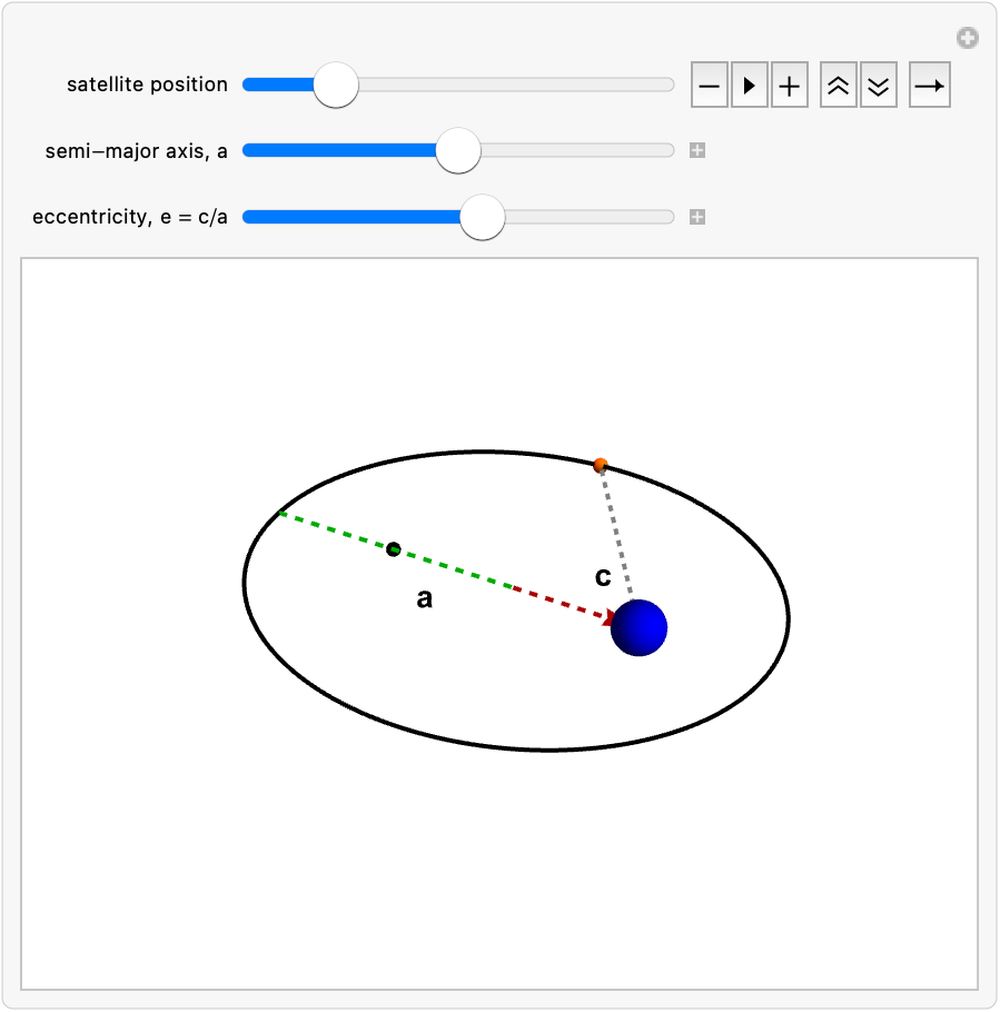
Kepler’s first law states: Planets move in elliptical orbits, with the sun at one of the two foci. The following diagram illustrates the geometry of a Keplerian satellite’s elliptical trajectory given in terms of the semimajor axis , eccentricity , focal length and inclination (see in later diagram). Their relationship is given by:
a
e
c
i

A Keplerian ellliptical orbit of a satellite with the earth at one of the two foci:
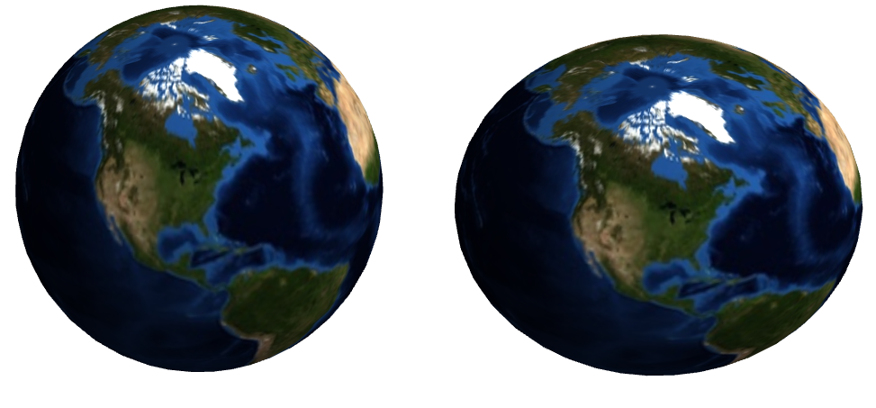
This model however is not completely accurate, as it assumes the Earth to be a perfect sphere. Practically speaking, however, Earth is an oblate spheroid.
Comparison of an unrealistic perfectly spherical Earth, with a more realistic oblate spheroid Earth:
Oblateness of the Earth
Oblateness of the Earth
Earth has a bulge at its equator, due to the centrifugal forces acting on it . This in turn results in a weaker gravitational field at the equator and thus the gravitational potential is no longer given by the simple formula:
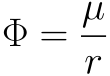
Instead, accounting for the earth’s oblateness we get:

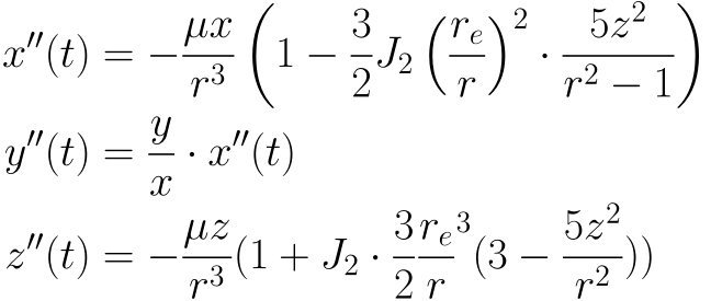
where are the Legendre polynomials obtained from Legendre’s differential equation, the equatorial radius of earth, the geocentric latitude and experimentally determined coefficients. The perturbation caused by the , the leading term in the expansion of the Legendre polynomials, forces a non-elliptic orbit . Hence, Kepler' s first law is no longer obeyed. From the potential, we can easily obtain the equations of motion given by:
P
n
r
E
L
J
n
J
n
Φ
Linear Flow on the Torus Model
Linear Flow on the Torus Model
Using the Best Mathematical Model
Using the Best Mathematical Model
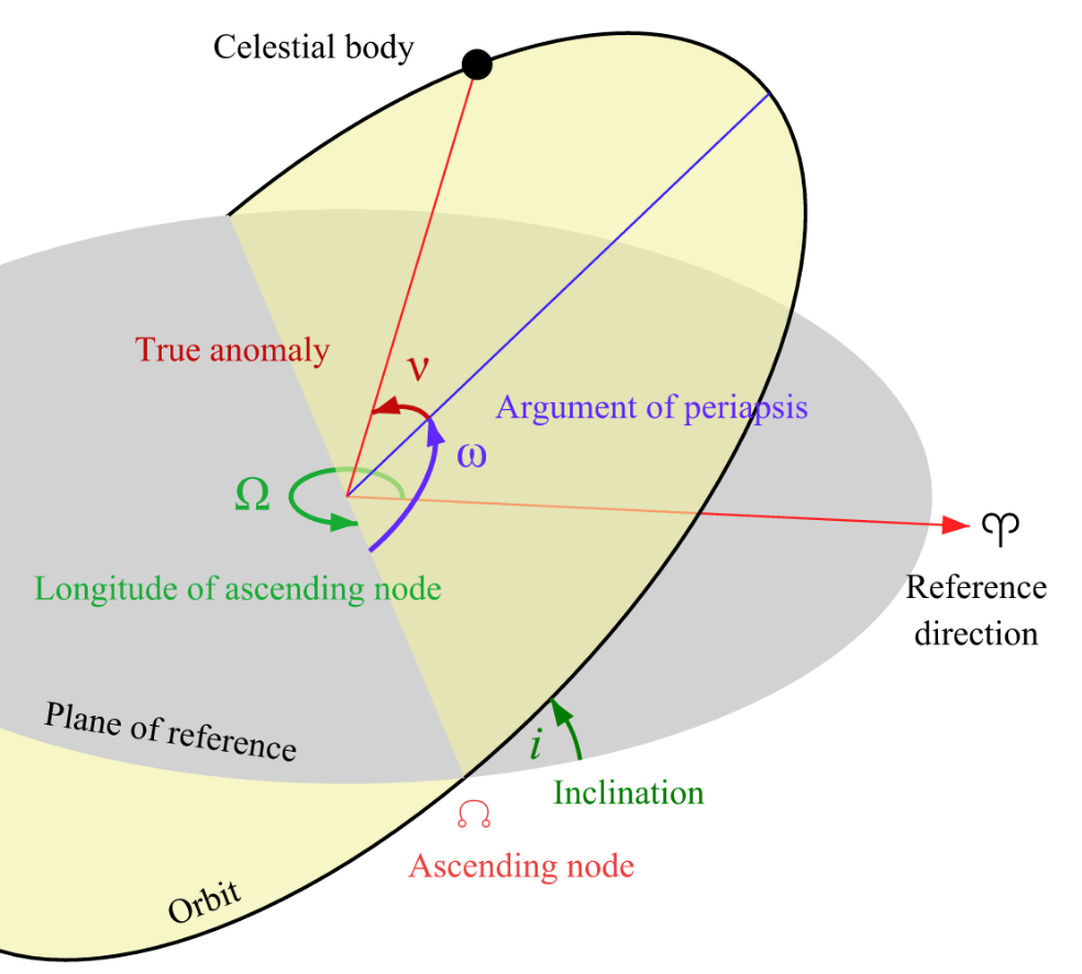
Keplerian orbits can be completely described by the following orbital element coordinates: where , semi-major axis, , eccentricity, , inclination, , Mean anomaly, , longitude of the ascending node and , argument of the periapsis. The first three orbital elements determine the geometry of the orbit and the last three elements determine the position of the satellite along that trajectory.
The mean anomaly can be obtained from the true anomaly (the angle between periapsis and the current satellite position), the longitude of the ascending node is the angle from the ascending node (where the trajectory intersects the plane of reference) and the argument of periapsis, gives the orientation of the elliptical orbit.
(a,e,i,M,Ω,ω)
a
e
i
M
Ω
ω
The mean anomaly
M
Ω
ω
Orbital elements diagram.Adapted from Snyder (2006), Wikimedia Commons. |
By integrating Lagrange planetary equations (obtained via the method of variations), we are able to deduce the following linearised flow equations:
Linear Flow on the Torus diagram:
What is Ergodicity?
What is Ergodicity?
Ergodic System
Ergodic System
Ergodic theory is the study of long-term behaviours of dynamical systems. In an Ergodic system if a single particle is tracked over a long-time frame, it will eventually visit every part of its state space regularly. We provide the classical example of a free particle in a box to demonstrate this phenomenon.
A simple example of ergodicity: Snapshots of particle position are taken at discrete time intervals T = 0, 1, ..., n
Time and Space Average: Bhirkoff-Khinchin theorem
Time and Space Average: Bhirkoff-Khinchin theorem
The left hand side is the time average which is the average value of the function evaluated along the trajectory of the satellite and the right hand side is the space average which is the average of the function over the entire state space. In the limit these two quantities are equal to each other.
Why do we consider our Satellite system to be ergodic?
Why do we consider our Satellite system to be ergodic?
◼
Important: A satellite orbit chosen at random can be shown to be ergodic with probability 1. Hence, satellite orbits are generically ergodic.
Ergodic vs. Non-Ergodic behaviour - the trajectory fills out the state space over long time periods:
Koksma-Hlawka inequality
Koksma-Hlawka inequality
The Number Theory connection
The Number Theory connection
Discrepancy of a sequence
Discrepancy of a sequence
The discrepancy of a sequence quantitatively measures how evenly distributed a sequence is. By evenly distributed we mean how close its distribution is to a uniformly distributed sequence. A sequence that is close to being uniformly distributed, is called a low discrepancy sequence and conversely a “non-uniformly “ distributed sequence is referred to as a high-discrepancy sequence. To visualize this, see on the left a low discrepancy sequence and on the right a high-discrepancy sequence.
Comparison of the discrepancy of two sequences:
Explicitly computing the discrepancy of a sequence is not typically possible, so the best one can do is to find an upper bound.
1-dimensional case: Continued Fractions
1-dimensional case: Continued Fractions
Lower dimensions : Brute Force approach
Lower dimensions : Brute Force approach
Higher dimensions: Curse of Dimensionality
Higher dimensions: Curse of Dimensionality
The following plots demonstrate how our computed discrepancy bound varies with the number of iterates:
Poincare sequence plots:
Floating Point Precision Problem
Floating Point Precision Problem
Connecting the dots: Computing the Probability of Collision
Connecting the dots: Computing the Probability of Collision
The probability of a satellite, being in a certain region is given by the proportion of flight time it spends in that region divided by the total flight time spends in its state space.
Ground Track of a Circular Orbit:
From the plot we see that the error bound is above the true error (the difference between the time and space average) and that the error bound converges to the discrepancy as expected .
Concluding Remarks
Concluding Remarks
The goal for this project was writing a paclet, such that when the user inputs the TLE’s of a pair of satellites, the suite of functions outputs the probability of collision, as well as the error margin of the collision probability. More precisely we have computed the discrepancy of a Kronecker sequence so as to obtain a bound via the Koksma-Hlawka inequality.
Acknowledgements
Acknowledgements
I would like to thank Alejandra Ortiz Duran, Pavel Hajek, and Dugan Hammock for all their help and support with this project. In addition I would like to thank Hugh Coleman for his numerous opinions on visualizations and Andrew Graven for his help in brainstorming ideas. Finally, I would like to thank Stephen Wolfram for his fruitful conversations.
References
References
This is our preferred reference style. You may use “et al.” if there are more than two authors.
1
.V. I. Arnold and A. Avez (1989), Ergodic Problems of Classical Mechanics. Addison-Wesley.
2
.K. F. Wakker (2015), Fundamentals of Astrodynamics. Delft University of Technology.
3
.D. A. Vallado (2013), Fundamentals of Astrodynamics and Applications, 4th ed., Microcosm Press.
4
.A. J. Graven et al. (2021), “A Rapid Method for Orbital Coverage Statistics with (J_2) Using Ergodic Theory,” AAS Space Flight Mechanics Meeting.
5
.L. Kuipers and H. Niederreiter (1974), Uniform Distribution of Sequences. John Wiley & Sons. Reprinted by Dover Publications in 2006.
6
.J.-C. Yoccoz (1992), “An Introduction to Small Divisor Problems,” in From Number Theory to Physics, edited by M. Waldschmidt, P. Moussa, J.-M. Luck, and C. Itzykson. Springer.
7
.M. Drmota and R. F. Tichy (2006), Sequences, Discrepancies and Applications. Springer.
AI Disclosure
AI Disclosure
The following generative AI tools were used in this project: ChatGPT 5.6. It was used for debugging code and helping generate images. All code and written content was reviewed, understood and approved by the author.
CITE THIS NOTEBOOK
CITE THIS NOTEBOOK
Estimating Satellite Collision Risk: An Ergodic Approach
by Leyla Sozen-Kohl
Wolfram Community, STAFF PICKS, July 16, 2026
https://community.wolfram.com/groups/-/m/t/3763243
by Leyla Sozen-Kohl
Wolfram Community, STAFF PICKS, July 16, 2026
https://community.wolfram.com/groups/-/m/t/3763243