Goal: Create a Wolfram Language function that take an arbitrary user-defined list of point light emitters and its experimental features as inputs and return the power spectrum of the non-paraxial interference/diffraction pattern produced under arbitrary phase and degree of spatial coherence.
Introduction
Introduction
Modeling non-paraxial optical fields at short propagation distances (comparable to the wavelength) is often considered a rather hard problem. The large non-paraxial propagation integral is a modal expansion that usually is computationally heavy due to its non-linear kernel, and most common algorithms can’t easily consider phase distributions and partially coherent light.
To solve this problem an algorithm was recently proposed. It is based on a theoretical framework that describes the screen or mask of a interference or diffraction experiment as a set of point light emitters using correlation functions. These points, called “real points”, are essentially little holes in the mask where the illuminating field is crossing. The correlation between every subset of two real points create the so-called “virtual points” that are located at the midpoint between the two real points, with each virtual point identified by its separation value and its support. These virtual points manage the spatial coherence of the field.
To solve this problem an algorithm was recently proposed. It is based on a theoretical framework that describes the screen or mask of a interference or diffraction experiment as a set of point light emitters using correlation functions. These points, called “real points”, are essentially little holes in the mask where the illuminating field is crossing. The correlation between every subset of two real points create the so-called “virtual points” that are located at the midpoint between the two real points, with each virtual point identified by its separation value and its support. These virtual points manage the spatial coherence of the field.
Real and virtual point array
Real and virtual point array
The task is to build a function that creates the virtual points array from a given array of 1D or 2D real points, and which can take a phase function and coherence function that specify respectively the phase of every real point and the coherence of every virtual point (based on its support). Considering the several possible syntaxes and logic to manage different structures and dimensions of the real points array, it is possible to create a PointArrayObject that contains all the data from the realPoints, the virtualPoints and the phase and coherence values derived from the phaseF and coherenceF functions.
Define a function that derives the phase of a virtual point from the phases of its constituent real points:
phaseOfPair=Function[{point1,point2},Apply[phaseF,point1]-Apply[phaseF,point2]];
For each subset of two real points, calculate the corresponding virtual point’s coordinates, support, and phase:
virtualPoints=Map[Join[Mean[#],Subtract@@#,{phaseOfPair@@#}]&,Subsets[realPoints,{2}]];
Apply the coherence function to each virtual point:
virtualPoints=Map[Join[#,{coherenceF@@Take[#,{3,4}]}]&,virtualPoints];
The OpticalFieldModeling function performs all of these operations and returns a PointArrayObject. This object stores an array of real points, an array of virtual points, and a vector describing the structure of the latter (which varies depending on whether phase and coherence functions have been specified):
In[]:=
pointArray=OpticalFieldModeling[N@CirclePoints[1,4]]
Out[]=
PointArrayObject


In[]:=
phaseF[ξA_]:=RandomReal[{0,2π}];OpticalFieldModeling[Range[-3,3],"PhaseFunction"phaseF]
Out[]=
PointArrayObject
In[]:=
σ=2;OpticalFieldModeling[Range[-3,3],"CoherenceFunction"PDF@MaxwellDistribution[σ]]
Out[]=
PointArrayObject
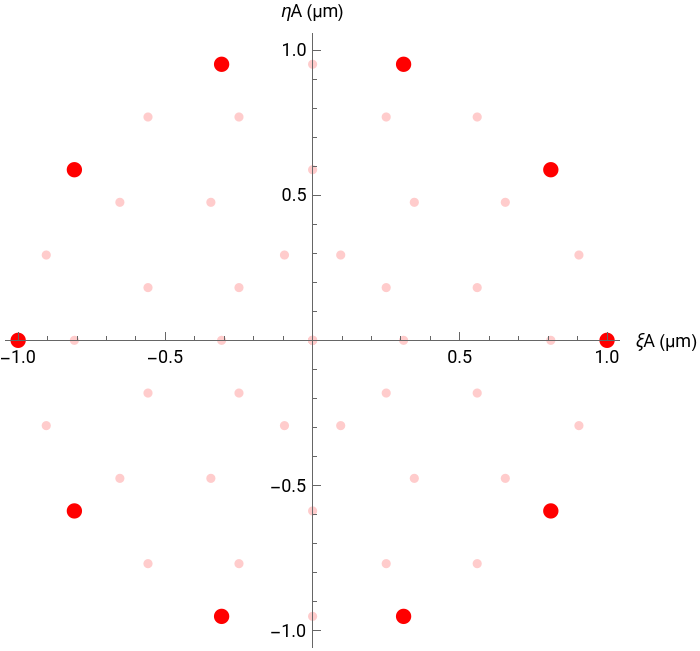
Sometimes is useful to be able to see the full array (both real and virtual points). The "PointPlot" property of the PointArrayObject plots the complete array, using for 2D arrays and for 1D arrays.
pointArray=OpticalFieldModeling[N@CirclePoints[1,10]];pointArray["PointPlot"]
Out[]=
The power spectrum
The power spectrum
Using the PointArrayObject we can calculate the resulting power spectrum (i.e. the energy distribution) for a given wavelength λ and propagation distance z. We do this using virtual point kernel and the real point kernel. These kernels calculate the energy contribution of each point which are then summed to produce the final power spectrum expression.
With the position coordinates (ξA,ηA), the kernel for the real points is given by:
1
4
2
λ
2
z+++
2
z
2
(x-ξA)
2
(y-ηA)
2
z
2
(x-ξA)
2
(y-ηA)
The kernel for the virtual points is given by:
μ
2
2
λ
z+++
2
z
2
x-ξA-
ξD
2
2
y-ηA-
ηD
2
2
z
2
x-ξA-
ξD
2
2
y-ηA-
ηD
2
z+++
2
z
2
x-ξA+
ξD
2
2
y-ηA+
ηD
2
2
z
2
x-ξA+
ξD
2
2
y-ηA+
ηD
2
2π
λ
2
z
2
x-ξA-
ξD
2
2
y-ηA-
ηD
2
2
z
2
x-ξA+
ξD
2
2
y-ηA+
ηD
2
Where μ is the complex degree of coherence and ϕ the phase difference between the two corresponding real points.
Applying these functions to the real and virtual points data, the "PowerSpectrum" property returns a PowerSpectrumObject containing the power spectrum expression:
Applying these functions to the real and virtual points data, the "PowerSpectrum" property returns a PowerSpectrumObject containing the power spectrum expression:
λ=0.632;(*Redlight*)z=10λ;(*6micrometers*)powerSpectrum=pointArray["PowerSpectrum",λ,z]
Out[]=
PowerSpectrumObject

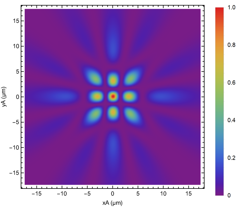
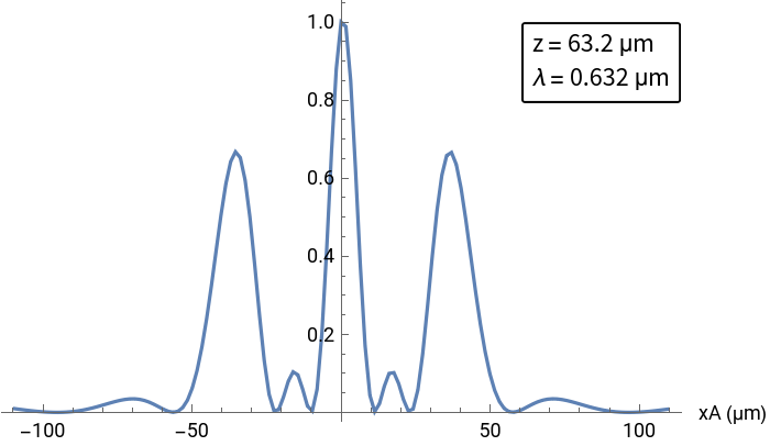
Finally, the power spectrum can be visualized for a given plotting angle and step in a one- or two-dimensional plot:
powerSpectrum["DensityPlot",70,step]
Out[]=
In[]:=
λ=0.632;pointArray1D=OpticalFieldModeling[N@Range[-2λ,2λ,2λ]];powerSpectrum1D=pointArray1D["PowerSpectrum",λ,100λ];powerSpectrum1D["Plot",60,1.6]
Out[]=
Results
Results
Using the OpticalFieldModeling function and associated objects’ properties, one can model complex and interesting experiments and physical phenomena, such as a speckle pattern, with just a few lines of code:
In[]:=
phaseF[ξA_,ηA_]:=RandomReal[{-π,π}];λ=0.632;speckleArray=OpticalFieldModeling[RandomPoint[Disk[{0,0},20λ],150],"PhaseFunction"phaseF];specklePS=speckleArray["PowerSpectrum",λ,1000λ];specklePS["DensityPlot",50,ColorFunctionGrayLevel]
Future work
Future work
A new version of the algorithm upon which this function is based is being developed. This will lead to the possibility of adding options to specify the local polarization angle, the mask’s transmittance, and the illuminating power spectrum. These additions will make the OpticalFieldModeling function more versatile, while still being able to simulate both near and far field without paraxial approximations under arbitrary conditions of spatial coherence.
Related links
Related links
Check my ResearchGate profile to read more about this algorithm!