Motivation
Motivation
Classical simulability refers to the ability to efficiently simulate the behavior of a quantum system using classical computers, which are based on classical bits and classical logic gates. Since those quantum circuits and algorithms which are classically simulable can be simulated with at best a polynomial overhead over the quantum algorithms, which themselves are riddled with the problems of noise, control, and scaling for the foreseeable future, quantifying the degree of ‘non-classical simulability’ is essential. Those algorithms with a high degree of ‘non-classical simulability’ can be said to be the most suitable algorithms for practical quantum advantage in the NISQ era. Generally this degree of ‘non-classical simulability’ is measured by the quantity of non-Cifford resources required (since, it has been established that Clifford gates or resources can be efficiently simulated classically) also popularly known as “magic”.
In this project I, with the help of my mentor Nikolay Murzin try to tackle this problem using two methods, one involves evaluating the quantum resource monotone of stabilizer Rényi entropy which measures the quantity of non-Clifford resources required. The other way involves creating a function which converts the QuantumCircuitOperator (quantum circuit) object to its corresponding ZX-diagram using the PyZX library. Once received the ZX-diagram can be analyzed if it must contain a spider outside of the Clifford fragment. If so, the circuit can not be simulated classically (efficiently). We provide two methods as borrowed from the PyZX library to simplify the circuit namely “Fuse” which fuses the spiders of same colors, and “Simplify” which simplifies the ZX-diagram leaving only green (Z) spiders.
Lastly we perform our evaluation on a Fourier Transform based quantum adder circuit which displays a non zero value of stabilizer Rényi entropy as well as contains a lot of spiders outside of the Clifford fragment. Although showing that a particular ZX diagram contains such spiders does not constitute as a proof. The non - zero values of the stabilizer Rényi entropy and the presence of spiders outside of the Clifford fragment in the fused and simplified circuits indicate that it is worth investigating in more details.
Stabilizer Rényi Entropy
Stabilizer Rényi Entropy
The stabilizer Rényi Entropy can be evaluated using the formula (3) below. The function is a standard resource monotone to measure the ‘nonstabilizerness’ or “magic” and is introduced at the following paper Stabilizer Rényi Entropy. The particular measure is easily computable since it does not need any minimization procedure as is claimed by the authors. The measure involves taking the sum of the trace of the state after the individual qubits have been acted upon by the strings of Pauli matrices. In particular we will be evaluating a particular form stabilizer Renyi Entropy with n = 2. The formula can be evaluated for other integer values of n by simply substituting the n values in the notebook with the appropriate value from (3). Note that the exponential phase in (1) does not matter since we will be taking the sums over the absolute values of the trace.


In this chapter we will create a function which evaluates the expression (3) and expression (1). We first create a function sumden which inputs a 3 qubit state and outputs its stabilizer Rényi entropy. Later we devise another function which is more generalizable to evaluate the stabilizer Rényi entropy of systems of different sizes. We evaluate the stabilizer Rényi entropy across the 3 qubit (total 6 qubits) and 4 qubit (total 8 qubits) Fourier Transform based adder circuits and plot the outputs.
Installing the WolframQuantumFramework Paclet
Installing the WolframQuantumFramework Paclet
First of all we will need to Install and verify the WolframQuantumFramework Paclet. The Paclet will allow us to construct various circuits and states, which are to be used in this notebook.
PacletInstall["Wolfram/QuantumFramework"]Needs["Wolfram`QuantumFramework`"]
Out[]=
PacletObject

We verify the installation by checking for all the functions are provided to us.
Names["Quantum*"]
Out[]=
{QuantumBasis,QuantumChannel,QuantumCircuitMultiwayCausalGraph,QuantumCircuitMultiwayGraph,QuantumCircuitOperator,QuantumCircuitPathGraph,QuantumCircuitTokenEventGraph,QuantumDistance,QuantumEntangledQ,QuantumEntanglementMonotone,QuantumEvolve,QuantumMeasurement,QuantumMeasurementOperator,QuantumMeasurementSimulation,QuantumMPO,QuantumMPS,QuantumOperator,QuantumPartialTrace,QuantumPartialTranspose,QuantumShortcut,QuantumState,QuantumStateEstimate,QuantumStateEstimation,QuantumStateSampler,QuantumTensorProduct,QuantumWeylTransform,QuantumWignerMICTransform,QuantumWignerTransform}
Calculating Stabilizer Rényi Entropy: Part 1
Calculating Stabilizer Rényi Entropy: Part 1
To create the sumden function which evaluates the stabilizer Rényi entropy we create a function which takes in input a number i and output the i_th Pauli matrix. This function will then be called by the others to get a Pauli matrix as needed. 0 is encoded to Identity, 1 is encoded to PauliX, 2 is encoded to PauliY, and 3 is encoded to PauliZ. We print the function to verify the assignments.
sig[arg_]:=Which[arg==0,IdentityMatrix[2],arg==1,PauliMatrix[1],arg==2,PauliMatrix[2],arg==3,PauliMatrix[3]]sig[0]//MatrixFormsig[1]//MatrixFormsig[2]//MatrixFormsig[3]//MatrixForm
Out[]//MatrixForm=
1 | 0 |
0 | 1 |
Out[]//MatrixForm=
0 | 1 |
1 | 0 |
Out[]//MatrixForm=
0 | - |
| 0 |
Out[]//MatrixForm=
1 | 0 |
0 | -1 |
Now we create a function called stringen[]. It generates an array of the tensor products of Pauli operators for 3 a qubit circuit as required by formula (1). For this we run 3 nested loops to create ordered 3 tuples. The sig[ ] function is then called which provides the appropriate Pauli matrix for the tuple entries. Lastly we do a tensor product of those Pauli matrices and store the final matrix in the list called strinarray.
In[]:=
stringen[]:=Module[{strinarray,strin},strinarray={};strin={0,0,0};For[i=0,i<4,i++,strin[[1]]=i;For[j=0,j<4,j++,strin[[2]]=j;For[k=0,k<4,k++,strin[[3]]=k;strinarray=Append[strinarray,KroneckerProduct[sig[strin[[1]]],sig[strin[[2]]],sig[strin[[3]]]]];]]];Return[strinarray];]
We execute the stringen[ ] function below which outputs all the matrices in the strinarray list. thus giving us all the matrices we need to evaluate the stabilizer Renyi entropy from formula (3).
stringen[]
Out[]//Short=
{{{1,0,0,0,0,0,0,0},{0,1,0,0,0,0,0,0},{0,0,1,0,0,0,0,0},{0,0,0,1,0,0,0,0},{0,0,0,0,1,0,0,0},{0,0,0,0,0,1,0,0},{0,0,0,0,0,0,1,0},{0,0,0,0,0,0,0,1}},{{0,1,0,0,0,0,0,0},{1,0,0,0,0,0,0,0},{0,0,0,1,0,0,0,0},{0,0,1,0,0,0,0,0},{0,0,0,0,0,1,0,0},{0,0,0,0,1,0,0,0},{0,0,0,0,0,0,0,1},{0,0,0,0,0,0,1,0}},{{0,-,0,0,0,0,0,0},{,0,0,0,0,0,0,0},{0,0,0,-,0,0,0,0},{0,0,,0,0,0,0,0},{0,0,0,0,0,-,0,0},{0,0,0,0,,0,0,0},{0,0,0,0,0,0,0,-},{0,0,0,0,0,0,,0}},58,{{0,1,0,0,0,0,0,0},{1,0,0,0,0,0,0,0},{0,0,0,-1,0,0,0,0},{0,0,-1,0,0,0,0,0},{0,0,0,0,0,-1,0,0},{0,0,0,0,-1,0,0,0},{0,0,0,0,0,0,0,1},{0,0,0,0,0,0,1,0}},{{0,-,0,0,0,0,0,0},{,0,0,0,0,0,0,0},{0,0,0,,0,0,0,0},{0,0,-,0,0,0,0,0},{0,0,0,0,0,,0,0},{0,0,0,0,-,0,0,0},{0,0,0,0,0,0,0,-},{0,0,0,0,0,0,,0}},{{1,0,0,0,0,0,0,0},{0,-1,0,0,0,0,0,0},{0,0,-1,0,0,0,0,0},{0,0,0,1,0,0,0,0},{0,0,0,0,-1,0,0,0},{0,0,0,0,0,1,0,0},{0,0,0,0,0,0,1,0},{0,0,0,0,0,0,0,-1}}}
Finally we create the sumden function. We use the stringen[ ] function as created above and execute formula (3). A list called stringenArray stores all the required matrices of form (1) and the sum of the trace of the products ρP where each P is picked from stringenArray. Using this form we evaluate the stabiliser Rényi entropy which is printed as the output.
In[]:=
sumden[den_]:=Module[{SRE,sum,i,result},sum=0;stringenArray=stringen[];For[i=1,i<=4^3,i++,sum=sum+Abs[Tr[den.stringenArray[[i]]]]^(4)/(2^3)];result=(1/(1-2))*Log2[N[sum]];Print[result]]
Evaluating the stabilizer Rényi Entropy for an example state. The example consists of a density matrix which is obtained by taking a tensor product of a “magic” state with the completely mixed state and produces 1 as the output indicating maximal stabilizer Renyi entropy as expected.
tempstate=QuantumCircuitOperator["Magic"][]["DensityMatrix"]magicstate=KroneckerProduct[tempstate,{{1/2,0},{0,1/2}}]sumden[magicstate]
Out[]=
SparseArray

Out[]=
SparseArray

1.
Creating Fourier Transform Based Adder
Creating Fourier Transform Based Adder
A quantum Fourier transform based adder works by Fourier transforming the first input e.g. ‘a’ to encode the data / value ‘a’ in the phase, and then using controlled phase shift gates with control on qubits of number b and target on Fourier transform of a to add a and b in the phase. Finally an inverse Quantum Fourier transform is done to receive a modular sum of a and b. To perform non-modular summation the size of the circuit must be 1 qubit larger than the size of the maximum input. In order to perform the quantum Fourier transform and control phase shift, Hadamard gates and controlled phase shift gates are needed.
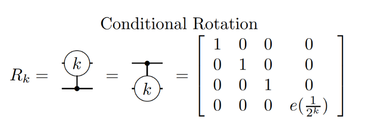
Below are the third ordered controlled phase shift and Hadamard gates. In general controlled phase shift of any order can be obtained by using appropriate integer in place of 3. the unitary for the controlled phase shift or a controlled rotation of order k looks like the following where e(x) = Exp[i*2πx]:
QuantumOperator[{"C","PhaseShift"[3]}]["Matrix"]//MatrixFormQuantumOperator[{"H"}]["Matrix"]//MatrixForm
Out[]//MatrixForm=
1 | 0 | 0 | 0 |
0 | 1 | 0 | 0 |
0 | 0 | 1 | 0 |
0 | 0 | 0 | π 4 |
Out[]//MatrixForm=
1 2 | 1 2 |
1 2 | - 1 2 |
3 Qubit Circuit
3 Qubit Circuit
We create an array of gates / operators named Oplist3 to be applied in a Fourier transformed based adder for 3 qubits. The arrangement of gates and why do they create a quantum Fourier transform is an interesting problem the solution to which can be found here or here. The inputs in the circuit are a = 7, and b = 7. The input is encoded using the X gates instead of the QuantumState function, this is to create a fixed circuit size from the beginning which will be needed later.
Oplist3={"X"->{1,2,3,4,5,6},"H"->1,{"C","PhaseShift"[2]}->{1,2},{"C","PhaseShift"[3]}->{1,3},"H"->2,{"C","PhaseShift"[2]}->{2,3},"H"->3,{"C","PhaseShift"[1]}->{1,4},{"C","PhaseShift"[2]}->{1,5},{"C","PhaseShift"[3]}->{1,6},{"C","PhaseShift"[1]}->{2,5},{"C","PhaseShift"[2]}->{2,6},{"C","PhaseShift"[1]}->{3,6},"H"->3,{"C","PhaseShift"[2]}->{2,3},"H"->2,{"C","PhaseShift"[3]}->{1,3},{"C","PhaseShift"[2]}->{1,2},"H"->1}
Out[]=
{X{1,2,3,4,5,6},H1,{C,PhaseShift[2]}{1,2},{C,PhaseShift[3]}{1,3},H2,{C,PhaseShift[2]}{2,3},H3,{C,PhaseShift[1]}{1,4},{C,PhaseShift[2]}{1,5},{C,PhaseShift[3]}{1,6},{C,PhaseShift[1]}{2,5},{C,PhaseShift[2]}{2,6},{C,PhaseShift[1]}{3,6},H3,{C,PhaseShift[2]}{2,3},H2,{C,PhaseShift[3]}{1,3},{C,PhaseShift[2]}{1,2},H1}
Passing the array of operators to the QuantumCircuitOperator function in order to create the QFT adder circuit on 3 qubits. Note that while we could have used the “Fourier” argument inside the QuantumOperator to create the same circuit more efficiently, we instead use an array of gates since we will be evaluating the stabilizer Rényi entropy after each gate has been applied to see how the values change across the circuit.
4 Qubit Circuit
4 Qubit Circuit
We create an array of gates / operators named Oplist4 to be applied in a Fourier transformed based adder for 4 qubits. The inputs are a = 15, and b = 15.
Passing the array of operators to the QuantumCircuitOperator function in order to create the QFT adder circuit on 4 qubits.
Extracting the States and Evaluating the function
Extracting the States and Evaluating the function
We extract the state of first 3 qubits from the 6 qubit circuit using the QuantumPartialTrace method after the fourier transform of the ‘a’ qubits has been performed, e.g., after 7 gates are executed from the Oplist3 array. The QuantumPartialTrace traces out the last 3 qubits namely qubit number 4, 5, and 6 and leaves the state of first 3 qubits. Note that for our particular case since the state is always a product state partial tracing over a qubit is equivalent to just ignoring the state of the qubit.
Similarly for the 8 qubit circuit we extract the state of first 4 qubits after the fourier transform of the ‘a’ qubits has been performed, e.g., after 11 gates are executed from the Oplist4 array.
Evaluating the sumden function over the reqmat3 state we see that the stabilizer Renyi entropy is non-zero as is expected. This indicates a non zero resource measure of “magic” and thus a state which can not be simulated classically in an efficient manner.
Now, we evaluate the sumden on the Fourier transform of state “111” using the Fourier argument inside the QuantumOperator and verify that we get the same value as above. However if we try to extract the state QuantumOperator[“Fourier”,3][QuantumState[“111”] we will find that the entries actually differ from what we have in the reqmat3 matrix. This is simply because the order of tensor product of qubits is opposite for the two states which can be corrected by the “SWAP” gate. However, such correction is not needed in the adder circuit because of the inverse Fourier transformation which corrects the order by flipping it again.
The sumden function however can not be easily tweaked to evaluate the stabilizer Rényi entropy of circuits of different number of qubits. This is because, for different number of qubits, different number of for loops will need to be nested inside the stringen[ ] function, which is then used by sumden. To avoid this predicament I had to learn about the StringJoin and Tuples functions using which we can create a more generalizable program to evaluate the stabilizer Rényi entropy.
Calculating Stabilizer Rényi Entropy: Part 2
Calculating Stabilizer Rényi Entropy: Part 2
A New Function to Calculate the monotone
A New Function to Calculate the monotone
The function uses Mathematica’s Tuples and StringJoin functions to easily create the array of the tensor product of the Pauli gates avoiding the need to create nested for loops. Then the stabilizer Rényi entropy is evaluated and printed. Below is the code which evaluates the function over 3 qubit input reqmat3.
Now we create the function to evaluate stabilizer Renyi entropy on 4 qubits and evaluate it over a 4 qubit input reqmat4 which is essentially the Fourier transformation of state “1111”. Non-zero value indicates the ‘non-classical simulability’.
Again verifying the function and the circuit by using the Fourier argument.
Evaluating stabilizer Rényi entropy across the whole circuit
Evaluating stabilizer Rényi entropy across the whole circuit
6 Qubit Circuit
6 Qubit Circuit
The following loop iterates over the Oplist3 array and finds the stabilizer Rényi entropy after the application of each unitary as the circuit progresses toward completion. All the values are iteratively stored in the list SREstring. The program also monitors the standard Rényi entropy values which will be printed and cleared below the cell once its executed. Here is why we used the “X” gates to encode states because the QuantumPartialTrace on the 6th qubit wont work unless the circuit itself has 6 qubits at all times.
Plotting stabilizer Renyi entropy (y-axis) as present after the appication of N_th gate in the circuit (x-axis) for the 6 qubit circuit.
8 Qubit Circuit
8 Qubit Circuit
The following loop iterates over the Oplist4 array and finds the stabilizer Rényi entropy after the application of each unitary as the circuit progresses toward completion. All the values are iteratively stored in the list SREstring2.
Plotting stabilizer Renyi entropy (y-axis) as present after the appication of N_th gate in the circuit (x-axis) for the 8 qubit circuit.
These bumps / non zero values of the standard Renyi entropy indicate a non-zero resource measure of “magic” or “nonstabilizerness” and thus creation of a state which may not be simulated classically in an efficient manner.
ZX-Diagrams
Of particular interest are the spiders with phase kπ/2 where k is an integers and the ZX-diagrams formed through these. All such ZX-diagrams constitute the Clifford fragment and it has been shown that all the Clifford gates can be constituted of the ZX-diagrams from the Clifford fragment. Therefore, If one can show that any ZX-diagram of a particular circuit (which is not unique) must contain a spider outside of the Clifford fragment then the circuit must have non-Clifford gate in any form providing it a non zero measure of the nonstabilizerness or the non classical simulability. What we are doing in the program below, therefore, is to create a function which can convert quantum circuits to ZX-diagrams, and simplifying it in various ways to check if the simplified ZX-diagrams contain spiders outside of the Clifford fragment.
Converting Quantum Circuits to ZX-Diagrams
Converting Quantum Circuits to ZX-Diagrams
The following function toZX[ ] takes a quantum circuit, more exactly a QuantumCircuitOperator object and converts it into a pyzx graph object i.e. a ZX-Diagram. The code first create python environment, loads Qiskit and converts the circuit in to a Qiskit QuantumCircuit object. Then it provides the QuantumCircuit object to PyZX which uses the .to_graph() method and outputs the graph object which carries the information to subsequently draw a string diagram. The function also has two arguments, Simplify” and, “Fuse”. Turning “Fuse” True fuses all the adjacent nodes of the same type using the fusion rule of ZX-Caculus and returns a simpler circuit. Similarly “Simplify” uses the simplify.full_reduce attribute of graph objects from pyzx and turning it True drastically simplify the ZX-diagram, leaving only Z-spiders and Hadamard boxes. All of the credit for the code goes to Nikolay.
We create the ZXTensorNetwork[ ] function using the toZX[ ] from above. It converts the output of the toZX[ ] function into a string diagram which is returned as a graphic.
Verifying the Packages:
Verifying the Packages:
We make sure that Qiskit is working by executing the following command.
Checking for Python Version. Make sure that the python version is 3.10 and above.
PyZX also should be installed in the same environment (v0.7.4 at least, which is only available on Github, released version has some QASM parsing bugs):
Examples:
Examples:
ZX-Diagrams of CRX gate
ZX-Diagrams of CRX gate
Here is the ZX-diagram for the above circuit with Simplify -> False and Fused -> False
ZX-diagram for the above circuit with Simplify -> False and Fused -> True
ZX-diagram for the above circuit with Simplify -> True.
The quantum circuit is first converted into a ZX diagram and them simplified to produce the following diagram.
The quantum circuit is first converted into a ZX diagram and them simplified to produce the following diagram.
ZX-diagram for the above circuit, with quantum circuit given without decomposition. We will show that all the 4 ZX diagrams correspond to the same tensor by using the ContractTensorNetwork function.
Resulting Tensors are Same!
Resulting Tensors are Same!
Here we print the resulting tensors and show that the 4 ZX diagrams above are actually the same.
Tensor for net0
Tensor for net2
Tensor for net3
Comparing to the actual tensor obtained through the “Tensor” method of QuantumOperator
It is evident that all the diagrams are producing the same tensor along with the “Tensor” method of QuantumOperator verifying that the ZXdiagrams so formed are correct and the simplification performed is also correct.
ZX-Diagrams of Toffoli gate
ZX-Diagrams of Toffoli gate
Here is the ZX-diagram for the Toffoli circuit with Simplify -> False and Fused -> False
ZX-diagram for the Toffoli circuit with Simplify -> False and Fused -> True
ZX-diagram for the Toffoli circuit with Simplify -> True
Quantum Fourier Transform
Quantum Fourier Transform
ZX-diagram for the QFT circuit on 3 qubits with Simplify -> False, and Fuse -> False
ZX-diagram for the QFT circuit on 3 qubits with Simplify -> False, and Fuse -> True
ZX-diagram for the QFT circuit on 3 qubits with Simplify -> True
Climax!
Climax!
We have finally reached the point where we will be converting the QFT based adder circuits to ZX diagrams :D
6 Qubit Circuit
6 Qubit Circuit
ZX-diagram for the QFT based adder circuit on 6 qubits with Simplify -> False, and Fuse -> False. Look at the many many spiders outside the Clifford fragment. Maybe we can reduce such spiders by fusing them using the fusion rule.
ZX-diagram for the QFT based adder circuit on 6 qubits with Simplify -> False, and Fuse -> True. Still many spiders outside of the Clifford fragment. Lets just simplify our circuit.
ZX-diagram for the QFT based adder circuit on 6 qubits with Simplify -> True. Looks like the non-Clifford spiders just wont go. Well, Just checking few of the simplified circuits certainly does not constitutes as a proof. However, from what we have here, getting rid of the non-Clifford spiders seems highly unlikely.
8 Qubit Circuit
8 Qubit Circuit
ZX-diagram for the QFT based adder circuit on 8 qubits with Simplify -> False, and Fuse -> False. The form is very similar to the 6 qubit circuit indeed with many spiders outside the Clifford fragment. Let us try to fuse them again.
ZX-diagram for the QFT based adder circuit on 8 qubits with Simplify -> False, and Fuse -> True. Again, many spiders outside of the Clifford fragment. Let us simplify for one last time.
ZX-diagram for the QFT based adder circuit on 8 qubits with Simplify -> True. The non-Clifford spiders prevailed after all.
So here we have done it. Now you know what those diagrams on the banner are and what they represent. We have created a the stabilizer Renyi entropy function, ran it across QFT based adder circuits, we have created a function to convert a quantum circuit in a ZX diagram and have shown that QFT based adders might love the non-Clifford spiders. To re-iterate however what we have shown is just that the QFT based adders are interesting and worth investigating into and not that their results are not classically simulable. A little investigation that I have done into them can be found at arXiv.
Future Works and Other Possibilities:
Future Works and Other Possibilities:
While the ZXTensorNetwork function above is really good at what it is doing (again, all credits to Nik) there is a possibility of creating and integrating many many ResourceFunctions in the WolframLanguage to support the ZX calculus framework. The first step might be to introduce functions which can execute the ZX rules. Subsequently one might try to create a network of ZX-diagrams related to each other by the ZX-rewrite rules, providing the ability to check for a certain property across a bunch of ZX-diagrams for the same circuit. For Quantum Magic many other resource monotones can be added, and the one we have provided might be improved upon.
Thank You!
Thank You!
Lastly it was a pleasure to participate in the winter school, with all the things I got to learn, and even more that I started to appreciate. Thank you to all the lecturer, mentors, my fellow participants, and to you the reader for engaging with this post.
References:
References:
CITE THIS NOTEBOOK
CITE THIS NOTEBOOK
Classical Simulability of Quantum Circuits Via Stabilizer Rényi Entropy and ZX-Diagrams
by Gaurang Agrawal
Wolfram Community, STAFF PICKS, January 11, 2024
https://community.wolfram.com/groups/-/m/t/3101026
by Gaurang Agrawal
Wolfram Community, STAFF PICKS, January 11, 2024
https://community.wolfram.com/groups/-/m/t/3101026