Adiabatic quantum computing provides an alternative paradigm for quantum algorithms, where the solution to a problem is encoded in the ground state of a final Hamiltonian. Instead of applying a sequence of quantum gates, the system is initialized in the ground state of a simple Hamiltonian and then slowly evolved toward a problem Hamiltonian whose ground state contains the desired answer.
In practical implementations, however, the success of the algorithm depends on spectral properties such as the minimum energy gap between the ground and first excited states and related quantities that bound the required evolution time.
In this post we illustrate these ideas with an extremely simple one-qubit example, using the Wolfram Quantum Framework to construct the Hamiltonians, visualize the spectral gap, estimate the adiabatic condition, and simulate the quantum evolution. Despite its simplicity, this example clearly shows how the spectral gap governs whether the adiabatic algorithm succeeds or fails, and how small perturbations on the system can dramatically affect the outcome.
Theory
Theory
According to the Adiabatic Quantum Computing (AQC) approach, a computational problem can be solved by evolving a quantum system from the ground state of a simple Hamiltonian to the ground state of another Hamiltonian that encodes the solution. The central idea is to let the system evolve under a Hamiltonian that slowly interpolates between an initial Hamiltonian and a problem Hamiltonian :
H
B
H
p
H(s)=(1-s)+s
H
B
H
P
How is this achieved?
Consider a quantum system that evolves according to:
|ψ(t)〉=H(t)|ψ(t)〉
t
Now define a smooth one-parameter family of Hamiltonians H(s):
H(t)=(t/T)=(s)
H
H
where
s=,s∈[0,1]
t
𝑇
The instantaneous eigenstates and eigenvalues of are defined by
H(s)
H(s)|l;s〉=(s)|l;s〉
E
l
with the energies ordered as
E
0
E
1
E
N-1
where is the dimension of the Hilbert space. If the system is initialized in the ground state of the initial Hamiltonian (0):
N
H
|(s=0)〉=|l=0;s=0〉
ψ
0
then the Adiabatic Theorem states that if the energy gap between the two lowest levels (s)-(s) remains strictly greater than zero for all , and the evolution time 𝑇 is sufficiently large, the system will remain arbitrarily close to the instantaneous ground state throughout the evolution:
E
1
E
0
0<=s<=1
𝑇->∞
l=0;s=1
ψ(𝑇)
This means that the existence of a nonzero gap ensures that the state |ψ(t)〉 remains arbitrarily close to the instantaneous ground state of H (s) throughout the process, provided that the total evolution time 𝑇 is sufficiently large compared to the inverse square of the minimum gap . Therefore, rather than exploring the Hilbert space arbitrarily, the system is constrained to follow the instantaneous ground state of H (s), starting from the ground state of Subscript[H, B] and ending in the ground state of Subscript[H, P], which encodes the solution to the computational problem.
A One-Qubit Adiabatic Example
A One-Qubit Adiabatic Example
Problem definition
Problem definition
Load the Wolfram Quantum Framework:
In[]:=
<<Wolfram`QuantumFramework`
Now we are ready to define the Hamiltonians required for this one-qubit problem.
Problem Hamiltonian
Problem Hamiltonian
We begin by defining the problem Hamiltonian , whose ground state encodes the desired solution:
H
P
In[]:=
Hp=(1+QuantumOperator["Z"])
1
2
Out[]=
|0〉〈0|
In this simple one-qubit example, the ground state corresponds to:
|1〉
In[]:=
Hp[QuantumState["1"]]
Out[]=
0
Initial Hamiltonian
Initial Hamiltonian
We also define an initial Hamiltonian , chosen such that its ground state is easy to prepare:
H
B
In[]:=
Hb=(1-QuantumOperator["X"])
1
2
Out[]=
1
2
1
2
1
2
1
2
In this case, the ground state is the superposition state :
|+〉
In[]:=
Hb[QuantumState["+"]]
Out[]=
0
So the algorithm should transform through a slow adiabatic evolution.
|+〉->|1〉
Interpolating Hamiltonian
Interpolating Hamiltonian
We define a smooth (slow evolution ) interpolating Hamiltonian:
s=t/T
In[]:=
H=QuantumOperator[(1-s)*Hb+s*Hp,"Parameters"->{s}]
Out[]=
1-s
2
1
2
1
2
1-s
2
This Hamiltonian gradually changes from to as goes from 0 to 1. This is exactly the Hamiltonian used during the adiabatic evolution.
H
B
H
P
s
Spectral analysis
Spectral analysis
To determine whether the adiabatic algorithm will successfully prepare the ground state of the problem Hamiltonian, it is useful to study the spectrum of the interpolating Hamiltonian during the evolution. In the adiabatic framework, the system evolves under a time-dependent Hamiltonian of the form , where As changes, the eigenvalues and eigenstates of also change continuously.
H(s)=(1-s)+s
H
B
H
P
sϵ[0,1].
s
H(s)
A key quantity is the spectral gap, defined as the difference between the lowest two eigenvalues of :
H(s)
g(s)=(s)-(s)
E
1
E
0
We calculate the eigenvalues (, ) from the QuantumOperator correspondent to the smooth interpolating Hamiltonian:
E
0
E
1
In[]:=
energies=H["Eigenvalues"]
Out[]=
1-1+
1
2
1-2s+2
,2
s
1
2
1-2s+2
2
s
According to the adiabatic theorem, the runtime required for the evolution to remain in the ground state depends inversely on the square of the minimum spectral gap encountered along the path. If this gap becomes very small or closes entirely the system can transition to excited states and the algorithm may fail to reach the desired solution.
By plotting the spectrum and identifying the minimum gap, we can anticipate whether the adiabatic evolution is likely to succeed and understand the role played by different choices of initial Hamiltonians or perturbations:
In[]:=
Plotenergies,{s,0,1},
Out[]=
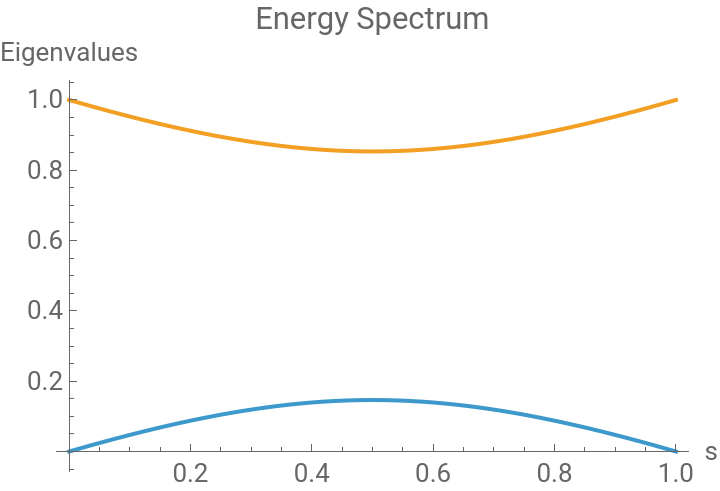


For this reason, analyzing how the eigenvalues of evolve as a function of provides important insight into the behavior of the algorithm. Now that we have visually determined that the gap is sufficiently large, we compute its actual value and plot it for
H(s)
s
s∈[0,1].
In[]:=
gap=Subtract@@Reverse@energies//Simplify
Out[]=
1-2s+2
2
s
In[]:=
Plotgap,{s,0,1},
Out[]=
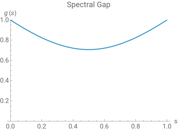
Compute the minimum gap, it determines how slow the evolution must be:
In[]:=
{gmin,smin}=FindMinimum[gap,s]
Out[]=
{0.707107,{s0.5}}
There are three important things to observe in these plots:
◼
Absence of level crossings.- This means >0, which is necessary for the adiabatic algorithm to succeed. If the levels cross, the ground state changes discontinuously and the system cannot follow it adiabatically.
g
min
◼
The minimum gap.- The gap becomes smallest near . This is the most critical point during the evolution. At this point the system is most likely to transition to the excited state.
s=0.5
◼
Physical interpretation.- When the gap becomes small, the ground and excited states are close in energy and the transitions between them become more likely. Therefore the evolution must be slower to avoid excitations.
Adiabatic condition
Adiabatic condition
While the minimum spectral gap provides an important indication of the difficulty of the evolution, it is not the only quantity that determines whether the adiabatic approximation holds. A more precise statement of the adiabatic condition involves the rate at which the Hamiltonian changes during the interpolation. In particular, the transition probability from the ground state to the first excited state depends on the matrix element:
1;s0;s
dH
ds
which measures how strongly the changing Hamiltonian couples the instantaneous ground state and the excited state. Then we define:
ξ=1;s0;s
max
0<=s<=1
dH
ds
This measures how strongly the Hamiltonian couples the ground state and the excited state during the evolution. The adiabatic theorem implies that the total evolution time 𝑇 must satisfy approximately:
𝑇>>
ξ
2
g
min
◼
g
min
◼
ξ:
In order to calculate ξ, we need to calculate the Hamiltonian eigenvectors:
In[]:=
{ψE0,ψE1}=QuantumState[#,"Parameters"->{s}]&/@H["Eigenvectors"]
Out[]=
0++11,0++11
s-
2-2s+1
2
s
(s-1)+1
2
s-
2-2s+1
2
s
s-1
1
2
s-
2-2s+1
2
s
s-1
s+
2-2s+1
2
s
(s-1)+1
2
s+
2-2s+1
2
s
s-1
1
2
s+
2-2s+1
2
s
s-1
Compute H derivative, then calculate and plot the ξ function:
Now we calculation the maximum value which correspond to ξ:
Simulating Adiabatic Evolution
Simulating Adiabatic Evolution
Using Instantaneous Eigenstates
Using Instantaneous Eigenstates
The results are consistent with the spectral analysis: since the minimum gap remains finite and the adiabatic condition is satisfied, the instantaneous ground state provides a continuous path toward the ground state of the problem Hamiltonian.
Using Evolution in Time
Using Evolution in Time
Similar to previous method, we found:
If the evolution time 𝑇 is sufficiently large, we observe:
Using a higher 𝑇 increase the result accuracy
Observe the improvement:
Methods comparison
Methods comparison
Gap Closing and Failure of the Adiabatic Algorithm
Gap Closing and Failure of the Adiabatic Algorithm
We now consider a slightly modified version of the previous example in order to illustrate a situation where the adiabatic algorithm fails. Since the procedure for constructing the interpolating Hamiltonian and analyzing its spectrum is the same as before, we focus only on the key differences that arise from this new choice of the initial Hamiltonian. As we will see, this modification introduces a symmetry that leads to a closing of the spectral gap, preventing the system from adiabatically reaching the ground state of the problem Hamiltonian.
Interpolating Hamiltonian
Interpolating Hamiltonian
We now construct the interpolating Hamiltonian for this modified case and examine its symmetry properties:
This symmetry is important because it prevents the Hamiltonian from coupling different basis states, so each state evolves independently. As a result, the energy levels can cross, leading to a vanishing spectral gap. As we saw in the previous section, the closing of the gap violates the conditions required for the system to remain in the instantaneous ground state.
Spectral analysis
Spectral analysis
In contrast with the previous example, the spectrum now exhibits a level crossing:
The two lowest eigenvalues intersect during the interpolation. As a result, the spectral gap closes at the crossing point, and the minimum gap satisfies:
The value of the spectral gap can be obtained directly from the difference between the two lowest eigenvalues along the interpolation:
Computing the minimum quantity confirms that the gap vanishes during the evolution:
Since the adiabatic condition requires a finite gap to prevent transitions to excited states, this level crossing prevents the system from reliably remaining in the instantaneous ground state throughout the evolution.
Evolution Simulation
Evolution Simulation
Now we evolve the system under the interpolating Hamiltonian to observe the behavior of the algorithm. In the previous spectral analysis we saw that the eigenvalues cross during the interpolation, which implies that the minimum spectral gap is zero. When the gap closes, the adiabatic condition cannot be satisfied, regardless of how slowly the system evolves.
Evaluating the final state shows that the probability distribution is exactly the same as the initial state:
In other words, the system ends in the same state in which it started. The adiabatic evolution fails to guide the system toward the ground state of the problem Hamiltonian. This result illustrates the consequence of the level crossing observed earlier: since the minimum spectral gap vanishes and the Hamiltonian remains diagonal in the same basis throughout the interpolation, the evolution cannot drive the system from the initial state to the desired solution state.
Reopen the Gap using Small Perturbation
Reopen the Gap using Small Perturbation
A simple way to resolve this issue is to introduce a small perturbation that breaks the symmetry. By adding a term that is not diagonal in the same basis, the degeneracy responsible for the level crossing is lifted. Physically, this perturbation mixes the states and prevents the eigenvalues from crossing, replacing the level crossing with an avoided crossing.
Interpolating Hamiltonian
Interpolating Hamiltonian
In the example discussed in the paper, this modification leads to the following interpolating Hamiltonian:
where ϵ is a small parameter controlling the strength of the perturbation. Even for small values of ϵ this term is enough to break the symmetry and produce a non-zero minimum gap.
Spectral analysis
Spectral analysis
In the following steps, we repeat the same analysis as before: we study the spectral structure of this Hamiltonian, compute the minimum gap, and verify through time evolution that the adiabatic algorithm now successfully reaches the ground state:
The effect of the perturbation can be clearly observed by varying the parameter ϵ :
As ϵ increases from zero, the degeneracy responsible for the level crossing is lifted and the eigenvalues separate, producing an avoided crossing. Even a small perturbation is sufficient to reopen the spectral gap, which is essential for the system to remain in the instantaneous ground state during the adiabatic evolution.
Adiabatic condition
Adiabatic condition
We now evaluate the adiabatic condition for the perturbed Hamiltonian. As in the previous section, we compute the quantity ξ:
Evolution simulation
Evolution simulation
Using instantaneous Eigenvectors
Using instantaneous Eigenvectors
Nevertheless, the key difference with the previous case is clear: the perturbation breaks the symmetry, opens a nonzero spectral gap, and enables the system to evolve away from the initial state and follow the instantaneous ground state toward the solution of the problem Hamiltonian.
Using evolution in time
Using evolution in time
◼
Evolution initialized from the Unperturbed Ground State:
◼
Evolution initialized from the initial Instantaneous Ground State
In summary, the success of adiabatic evolution critically depends on the presence of a finite spectral gap. When the Hamiltonian remains diagonal in a fixed basis, level crossings lead to a vanishing gap and prevent the system from reaching the desired solution. In contrast, even a small perturbation introduces coupling between states, lifts the degeneracy, and restores a finite gap, allowing the system to follow the instantaneous ground state and successfully reach the solution of the problem Hamiltonian.
Conclusions
Conclusions
In this work, we implemented a minimal example of Adiabatic Quantum Computing following the framework introduced by Farhi et al. By analyzing the interpolating Hamiltonian H(s), we showed how the spectral properties, particularly the minimum gap, determine the success of the algorithm.
Through the study of instantaneous eigenstates, we visualized the adiabatic path connecting the initial and final ground states, and complemented this analysis with explicit time evolution using QuantumEvolve. We also examined a failure case where the gap closes due to symmetry, and demonstrated how a small perturbation restores a finite gap and enables the algorithm to succeed.
This example illustrates, in a simple setting, the key mechanisms underlying adiabatic quantum computation and highlights the central role of the spectral gap in guiding the evolution toward the desired solution.
References
References
◼
Farhi, E., Goldstone, J., Gutmann, S., & Sipser, M. (2000). Quantum Computation by Adiabatic Evolution (Version 1). arXiv. https://doi.org/10.48550/ARXIV.QUANT-PH/0001106
◼
Brady, L. T., & van Dam, W. (2016). Spectral-gap analysis for efficient tunneling in quantum adiabatic optimization. Physical Review A, 94(3). https://doi.org/10.1103/physreva.94.032309
CITE THIS NOTEBOOK
CITE THIS NOTEBOOK
Adiabatic quantum computing: spectral analysis and simulation of a one-qubit system
by Sebastian Rodriguez
Wolfram Community, STAFF PICKS, March 31, 2026
https://community.wolfram.com/groups/-/m/t/3672532
by Sebastian Rodriguez
Wolfram Community, STAFF PICKS, March 31, 2026
https://community.wolfram.com/groups/-/m/t/3672532