Introduction
Introduction
◼
Happy Pi Day! Today (3/14) we celebrate the most famous mathematical constant: π ≈ 3.141592653589793…
◼
π is irrational and transcendental, appears in circles, waves, probability, physics, and even random walks.
◼
Wolfram Language (with its built-in π constant, excellent rational support, symbolic programming, and vast collection of Number Theory functions) makes experimenting with π especially easy and enjoyable.
◼
In this notebook we explore a selection of formulas and algorithms.
1. Continued fraction approximation
1. Continued fraction approximation
The built-in Wolfram Language (WL) constant Pi (or π ) can be computed to an arbitrary high precision:
In[]:=
N[Pi,60]
Out[]=
3.14159265358979323846264338327950288419716939937510582097494
Let us compare it with a continued fraction approximation. For example, using the (first) sequence line of On-line Encyclopedia of Integer Sequences (OEIS) A001203 produces π with precision 100:
In[]:=
s={3,7,15,1,292,1,1,1,2,1,3,1,14,2,1,1,2,2,2,2,1,84,2,1,1,15,3,13,1,4,2,6,6,99,1,2,2,6,3,5,1,1,6,8,1,7,1,2,3,7,1,2,1,1,12,1,1,1,3,1,1,8,1,1,2,1,6,1,1,5,2,2,3,1,2,4,4,16,1,161,45,1,22,1,2,2,1,4,1,2,24,1,2,1,3,1,2,1};N[FromContinuedFraction[s],120]
Out[]=
3.14159265358979323846264338327950288419716939937510582097494459230781640628620899862803482534211706808656553677697242141
Here we verify the precision using Wolfram Language:
In[]:=
N[Pi,200]-%
Out[]=
-1.0441745026369011477×
-100
10
2. Continued fraction terms plots
2. Continued fraction terms plots
It is interesting to consider the plotting the terms of continued fraction terms of \pi .
In[]:=
terms=Partition[ToExpression/@StringSplit[Import["https://oeis.org/A001203/b001203.txt"],Whitespace],2]〚All,2〛;Length[terms]
Out[]=
20000
Here is the summary:
In[]:=
ResourceFunction["RecordsSummary"][terms]
Out[]=
1 column 1 | ||||||||||||
|
Here is an array plot of the first 128 terms of the continued fraction approximating \pi :
In[]:=
mat=IntegerDigits[terms〚1;;128〛,2];maxDigits=Max[Length/@mat];mat=Map[Join[Table[0,maxDigits-Length[#]],#]&,mat];
In[]:=
ArrayPlot[Transpose[mat],Mesh->True,ImageSize->1000]
Out[]=

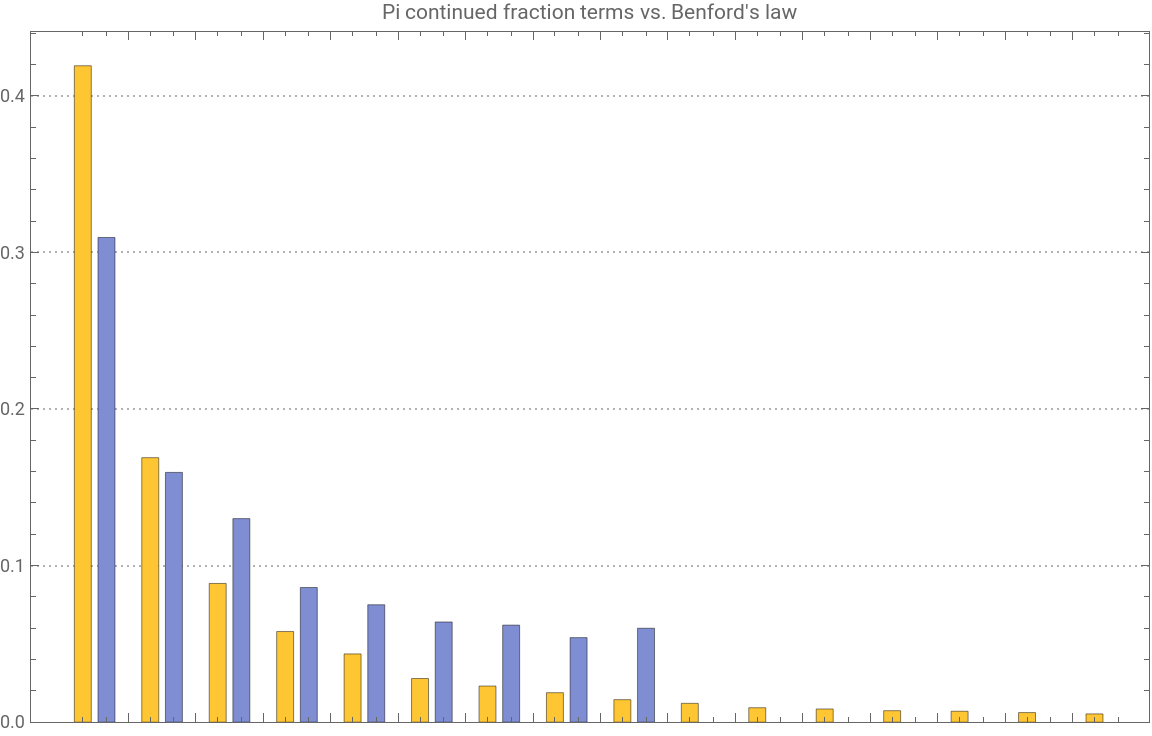
Next, we show the Pareto principle manifestation of for the continued fraction terms. First we observe that the terms a distribution similar to Benford's law :
In[]:=
tallyPi=KeySort[AssociationThread@@Transpose[Tally[terms]]]〚1;;16〛/Length[terms];
In[]:=
termsB=RandomVariate[BenfordDistribution[10],2000];tallyB=KeySort[AssociationThread@@Transpose[Tally[termsB]]]/Length[termsB];
In[]:=
data={tallyPi,tallyB};data=KeySort/@Map[KeyMap[ToExpression,#]&,data];data2=First/@Values@Merge[{data〚1〛,Join[AssociationThread[Keys[data〚1〛],Null],data〚2〛]},List];
BarChartdata2,
Out[]=


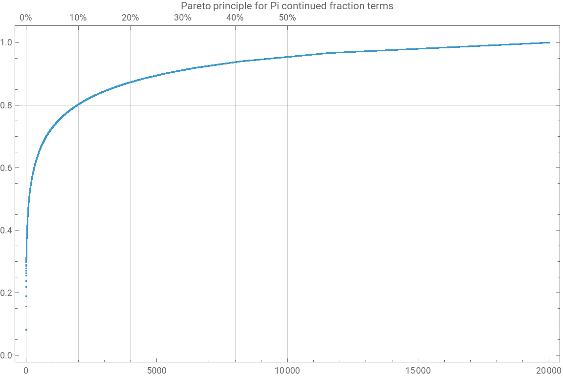
Here is the Pareto principle plot -- ≈5% of the unique term values correspond to ≈80% of the terms:
ResourceFunction["ParetoPrinciplePlot"]terms,
Out[]=
3. Classic Infinite Series
3. Classic Infinite Series
Many ways to express π as an infinite sum — some converge slowly, others surprisingly fast.
Leibniz–Gregory series (1671/ Madhava earlier)
π4=41-+-+⋯
∞
∑
n=0
n
(-1)
2n+1
1
3
1
5
1
7
WL implementation:
In[]:=
PiLeibniz[n_Integer]:=Block{},4*TotalTable(2i+1),{i,0,n-1}
i
(-1)
In[]:=
N[PiLeibniz[1000],20]
Out[]=
3.1405926538397929260
Verify with Wolfram Language (again):
In[]:=
N[Pi,100]-N[PiLeibniz[1000],1000]
Out[]=
0.000999999750000312499046880410106913745780068595381331607486808765908475046461390362862493334446861
π=3+·4
∞
∑
n=1
1+n
(-1)
2n(1+2n)(2+2n)
WL:
In[]:=
PiNilakantha[n_Integer]:=Block{},3+4*TotalTable(2i(2i+1)(2i+2)),{i,1,n}
(i+1)
(-1)
In[]:=
N[PiNilakantha[1000],20]
Out[]=
3.1415926533405420519
In[]:=
N[Pi,40]-N[PiNilakantha[1000],40]
Out[]=
2.49251186562514647026299317045×
-10
10
3. Beautiful Products
3. Beautiful Products
π
2
∞
∏
n=1
2
(2n)
(2n-1)(2n+1)
2×2×4×4×6×6⋯
3×3×5×5×7
WL running product:
p=2.0;Do[p*=(2n)^2/((2n-1)(2n+1));If[Divisible[n,100],Print[Row[{n," → ",p/π," relative error"}]]],{n,1,1000}]
4. Very Fast Modern Series — Chudnovsky Algorithm
4. Very Fast Modern Series — Chudnovsky Algorithm
One of the fastest-converging series used in record computations:
Each term adds roughly 14 correct digits.
5. Spigot Algorithms — Digits “Drip” One by One
5. Spigot Algorithms — Digits “Drip” One by One
Spigot algorithms compute decimal digits using only integer arithmetic — no floating-point errors accumulate.
The classic Rabinowitz–Wagon spigot (based on a transformed Wallis product) produces base-10 digits sequentially.
Simple (but bounded) version outline in WL:
Bailey–Borwein–Plouffe (1995) formula lets you compute the n-th hexadecimal digit of π directly (without earlier digits):
WL snippet for partial sum (base 16 sense):
7. (Instead of) Conclusion
7. (Instead of) Conclusion
◼
π contains (almost surely) every finite sequence of digits — your birthday appears infinitely often.
◼
The Feynman point : six consecutive 9s starting at digit 762.
◼
Memorization world record > 100,000 digits.
◼
π appears in the normal distribution, quantum mechanics, random walks, Buffon's needle problem (probability ≈ 2/π).
Let us plot a “random walk” using the terms of continued fraction of Pi -- the 20k or OEIS A001203 -- to determine directions:
Here is a bubble chart based on the path points and term values:
Remark: The bubble sizes indicate that some of terms are fairly large, but the majority of them are relatively small.
Here is a 3D point plot with of moving average of the 3D path modified to have the logarithms of the term values:
References
References
CITE THIS NOTEBOOK
CITE THIS NOTEBOOK
Pi Day 2026: formulas, series, and plots for π
by Anton Antonov
Wolfram Community, STAFF PICKS, March 14, 2026
https://community.wolfram.com/groups/-/m/t/3661100
by Anton Antonov
Wolfram Community, STAFF PICKS, March 14, 2026
https://community.wolfram.com/groups/-/m/t/3661100