Lagrange Multipliers in Two Dimensions
Lagrange Multipliers in Two Dimensions


This Demonstration intends to show how Lagrange multipliers work in two dimensions.
The 1D problem, which is simpler to visualize and contains some essential features of Lagrange multipliers, is treated in another Demonstration that can serve as an introduction to this one.
Details
Details
The main ideas behind the Lagrange multipliers have already been discussed in the 1D case. See Lagrange Multipliers in One Dimension.
This Demonstration illustrates the 2D case, where in particular, the Lagrange multiplier is shown to modify not only the relative slopes of the function to be minimized and the rescaled constraint (which was already shown in the 1D case), but also their relative orientations (which do not exist in the 1D case).
λ
f
λR
This in turn shows how the independence of and is restored by the introduction of (which is adjusted so that and are strictly parallel in both slope and orientation, so that their height difference remains constant near the solution, with no more constraint between and ).
x
y
λ
f
λR
F
x
y
The global problem can be understood as finding a point that is:
1. on the particular contour line , and
R(x,y)=K
2. on a contour line or (the constant is unknown, as the contour line is what we are looking for) tangent to the previous one.
f(x,y)=constant
df=0
By imposing (for any ), we impose that and share the same orientation but with different relative slopes (depending on ).
gradf(x,y)=λgradR(x,y)
λ
f(x,y)
λR(x,y)
λ
λ
f(x,y)
λR(x,y)
f-λR
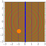
Here are a few explanations for each of the four plots displayed:
• upper-left: this is the case treated without the Lagrange multiplier. The thick blue line is the constraint, the thick red line is its projection on , and the solution is the top of the red thick line.
f
• upper-right: this is the case treated with the help of . The constraint function is rescaled (), but as , the constraint (thick blue line) keeps the same position as in the previous case. The function plotted in green is the new potential, which is to be optimized without constraint on . When equilibrium is forced, its extremum corresponds to the solution of the problem. When equilibrium is not forced, it is a function of the three variables , , .
λ
R
λR
λR=λK
F
(x,y)
x
y
λ
• bottom-left: same as upper-right, but with a contour representation, which shows more clearly the contour lines and the extremums of the three functions involved. The orange point is the one given by the 2D slider. When equilibrium is forced, it shows the solution of the problem (top of the green function ); otherwise it can be used to explore the slopes with the bottom-right panel.
F
• bottom-right: this is a close-up (tangent planes) of the plots of the three functions involved around the position (orange point) chosen by the 2D slider. It allows a comparison between their slopes. In particular, when , and have the same orientation but different slopes (this amounts to the 1D problem), and near the solution, they become completely parallel. When , their orientations are different. When equilibrium is forced, their slopes remain parallel, hence remains horizontal (constant).
y=0
f
λR
y≠0
F
When forcing equilibrium, you can only change (then , , and are the computed unique solution of the problem).
K
λ
x
y
With the equilibrium box unchecked, you can change (a slider) and (2D slider) to get a feeling of how they act and what they mean.
λ
(x,y)
External Links
External Links
Permanent Citation
Permanent Citation
Cedric Voisin
"Lagrange Multipliers in Two Dimensions"
http://demonstrations.wolfram.com/LagrangeMultipliersInTwoDimensions/
Wolfram Demonstrations Project
Published: July 18, 2012