Thermodynamic Study of Coal-Steam Gasification using Gibbs Free Minimization
Authors: Housam Binous, Raoudha Garma and Ahmed Bellagi
Thermodynamic Study of Coal-Steam Gasification using Gibbs Free Minimization
Authors: Housam Binous, Raoudha Garma and Ahmed Bellagi
Authors: Housam Binous, Raoudha Garma and Ahmed Bellagi
References :[1] S. I. Sandler, Chemical, Biochemical and Engineering Thermodynamics, 5th Edition, NY: Wiley, 2017.[2] Tilouche, R., Garma, R., Binous, H. et al. Valorization of Tunisian olive pomace by steam gasification: thermodynamic study using MATHEMATICA© and ASPEN-PLUS®. Biomass Conv. Bioref. (2023). https://doi.org/10.1007/s13399-023-04167-z[3] https://webbook.nist.gov/chemistry[4] Barin I. Thermochemical Data of Pure Substances. 3rd ed. VCH Verlagsgesellschaft; 1995.
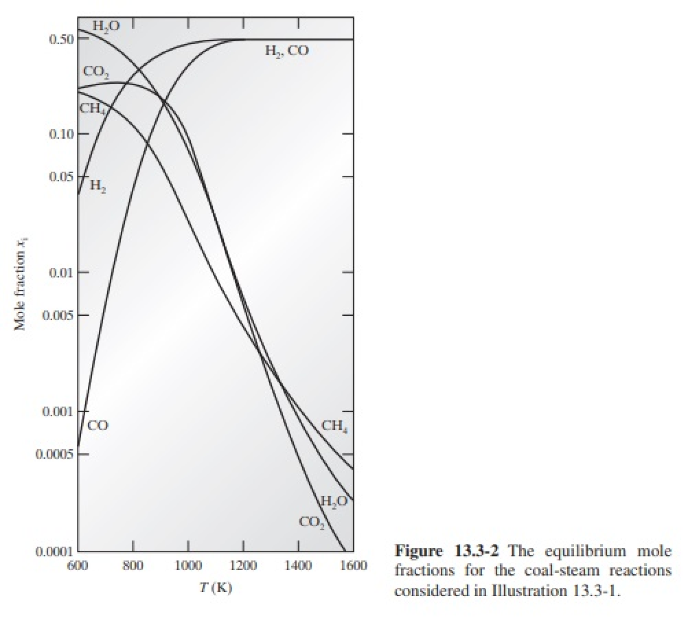
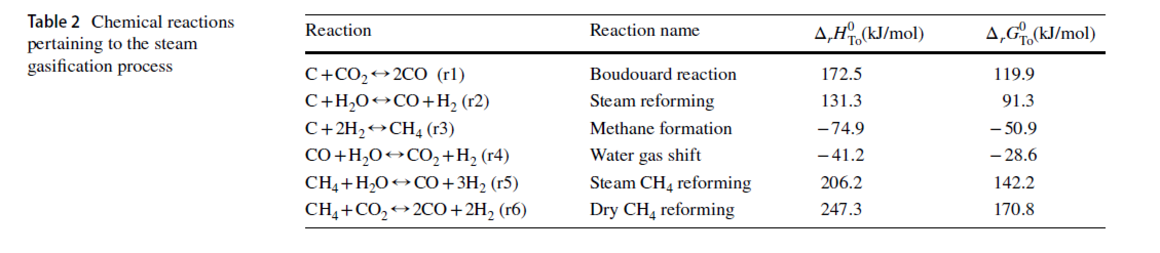
We compute the equilibrium mole fractions of H2O, CO, CO2, H2, and CH4 in the steam-carbon system at a total pressure of 1 bar and over the temperature range of 600 to 1600 K.Reaction taking place at 1 Bar (Ref. 2) :We Minimize the Gibbs free energy of the mixture subject to the following elemental conservation constraints:C : n_CH4 + n_CO + n_CO2 + n_C = 10 or any large value!!!H : 4*n_CH4 + 2*n_H2 + 2*n_H2O = 2 O : n_H2O + n_CO + 2*n_CO2 = 1
In[]:=
Off[General::"spell1"]
Gibbs free energy versus temperature are obtained using NIST Chemistry WebBook (Ref. 2 and 3) and Barin’s textbook (Ref. 4 for carbon)
In[]:=
Gwater[T_]:=Modulea,b,c,d,e,f,g,h,θ=,ΔHo=-241.826,HH,SS,If[500≤T≤1700,{a,b,c,d,e,f,g,h}={30.09200,6.832514,6.793435,-2.534480,0.082139,-250.8810,223.3967,-241.8264},If[1700<T≤6000,{a,b,c,d,e,f,g,h}={41.96426,8.622053,-1.499781,0.098119,-11.15764,-272.1797,219.7809,-241.8264}]];HH=aθ+++-+f-h+ΔHo;SS=;HH-TSS
T
1000
b
2
2
θ
c
3
3
θ
d
4
4
θ
e
θ
aLog[θ]+bθ++-+g
c
2
2
θ
d
3
3
θ
e
2
2
θ
1000
In[]:=
Gh2[T_]:=Modulea,b,c,d,e,f,g,h,θ=,ΔHo=0.0,HH,SS,If[298<T≤1000,{a,b,c,d,e,f,g,h}={33.066178,-11.363417,11.432816,-2.772874,-0.158558,-9.980797,172.707974,0.0},If[1000≤T≤2500,{a,b,c,d,e,f,g,h}={18.563083,12.257357,-2.859786,0.268238,1.977990,-1.147438,156.288133,0.0},If[2500<T≤6000,{a,b,c,d,e,f,g,h}={43.413560,-4.293079,1.272428,-0.096876,-20.533862,-38.515158,162.081354,0.0}]]];HH=aθ+++-+f-h+ΔHo;SS=;HH-TSS
T
1000
b
2
2
θ
c
3
3
θ
d
4
4
θ
e
θ
aLog[θ]+bθ++-+g
c
2
2
θ
d
3
3
θ
e
2
2
θ
1000
In[]:=
Gco[T_]:=Modulea,b,c,d,e,f,g,h,θ=,ΔHo=-110.53,HH,SS,If[298≤T≤1300,{a,b,c,d,e,f,g,h}={25.56759,6.096130,4.054656,-2.671301,0.131021,-118.0089,227.3665,-110.5271},If[1300<T≤6000,{a,b,c,d,e,f,g,h}={35.15070,1.300095,-0.205921,0.013550,-3.282780,-127.8375,231.7120,-110.5271}]];HH=aθ+++-+f-h+ΔHo;SS=;HH-TSS
T
1000
b
2
2
θ
c
3
3
θ
d
4
4
θ
e
θ
aLog[θ]+bθ++-+g
c
2
2
θ
d
3
3
θ
e
2
2
θ
1000
In[]:=
Gco2[T_]:=Modulea,b,c,d,e,f,g,h,θ=,ΔHo=-393.51,HH,SS,If[298≤T≤1200,{a,b,c,d,e,f,g,h}={24.99735,55.18696,-33.69137,7.948387,-0.136638,-403.6075,228.2431,-393.5224},If[1200<T≤6000,{a,b,c,d,e,f,g,h}={58.16639,2.720074,-0.492289,0.038844,-6.447293,-425.9186,263.6125,-393.5224}]];HH=aθ+++-+f-h+ΔHo;SS=;HH-TSS
T
1000
b
2
2
θ
c
3
3
θ
d
4
4
θ
e
θ
aLog[θ]+bθ++-+g
c
2
2
θ
d
3
3
θ
e
2
2
θ
1000
In[]:=
Gch4[T_]:=Modulea,b,c,d,e,f,g,h,θ=,ΔHo=-74.87,HH,SS,If[298≤T≤1300,{a,b,c,d,e,f,g,h}={-0.703029,108.4773,-42.52157,5.862788,0.678565,-76.84376,158.7163,-74.87310},If[1300<T≤6000,{a,b,c,d,e,f,g,h}={85.81217,11.26467,-2.114146,0.138190,-26.42221,-153.5327,224.4143,-74.87310}]];HH=aθ+++-+f-h+ΔHo;SS=;HH-TSS
T
1000
b
2
2
θ
c
3
3
θ
d
4
4
θ
e
θ
aLog[θ]+bθ++-+g
c
2
2
θ
d
3
3
θ
e
2
2
θ
1000
In[]:=
Tc=Join[{298.15},Table[i,{i,300,2000,100}]];
In[]:=
Gs=Interpolation[Transpose[{Tc,{-1.712,-1.722,-2.449,-3.473,-4.789,-6.386,-8.248,-10.358,-12.700,-15.257,-18.016,-20.965,-24.091,-27.385,-30.837,-34.439,-38.183,-42.061,-46.069}}]];
In[]:=
P=P1;P1=1;
In[]:=
y[i_]:=n[i]/Sum[n[j],{j,1,5}]/.n[1]n1/.n[2]n2/.n[3]n3/.n[4]n4/.n[5]n5/.n[6]n6
In[]:=
G[x_,P_,1]:=10^3Gch4[x]+RxLog[P/P1];G[x_,P_,2]:=10^3Gh2[x]+RxLog[P/P1];G[x_,P_,3]:=10^3Gwater[x]+RxLog[P/P1];G[x_,P_,4]:=10^3Gco[x]+RxLog[P/P1];G[x_,P_,5]:=10^3Gco2[x]+RxLog[P/P1];
In[]:=
Gtot[x_,P_]:=Sum[n[j]*(G[x,P,j]+RxLog[n[j]/Sum[n[k],{k,1,5}]]),{j,1,5}]+10^3Max[{n[6],0}]*Gs[x];
In[]:=
R=8.314;
In[]:=
sol[x_]:=Minimize[{Re[Gtot[x,P]],(n[1]+n[5]+n[4]+Max[{n[6],0}]10),(4n[1]+2n[2]+2n[3]2),(n[3]+n[4]+2n[5]1),0<n[1],0<n[2],0<n[3],0<n[4],0<n[5],0<n[6]}/.n[1]n1/.n[2]n2/.n[3]n3/.n[4]n4/.n[5]n5/.n[6]n6,{n1,n2,n3,n4,n5,n6}][[2]]
In[]:=
T=600;i=0;While[T<1610,{SOL=sol[T],tbl[i]=Table[y[i]/.SOL,{i,1,5}],Tp[i]=T,T=T+20,i=i+1}]
In[]:=
tbl1=Table[{Tp[i],tbl[i][[1]]},{i,0,50}];
In[]:=
tbl2=Table[{Tp[i],tbl[i][[2]]},{i,0,50}];
In[]:=
tbl3=Table[{Tp[i],tbl[i][[3]]},{i,0,50}];
In[]:=
tbl4=Table[{Tp[i],tbl[i][[4]]},{i,0,50}];
In[]:=
tbl5=Table[{Tp[i],tbl[i][[5]]},{i,0,50}];
Plotting the equilibrium mole fractions for the coal steam reactions.
Comparison between our data (colord lines) and the digitized data (black squares) from Fig. 13.3 - 2 (Ref. 1)