An adaptive-mesh PDE solver with potential connections to The Wolfram Model
By Omid Mozafar
University of Ottawa
By Omid Mozafar
University of Ottawa
The Finite Volume Method (FVM) is an increasingly popular numerical scheme, well suited for solving partial differential equations (PDEs), particularly those representing conservation laws. The FVM is based on the integral form of PDEs, which is often how these equations are derived from their associated physical laws. This method can be instantiated on physical spaces modeled as unstructured meshes, which accommodate the irregularly shaped boundaries and the scheme itself is locally adaptive, leading to high resolution structures. This project aims at developing a 1D numerical PDE solver algorithm based on the FVM, in particular, the FORCE scheme, formulated on adaptive meshes to solve the 1D time-dependent advection equation. The novelty of this work lies in using the limited slope criterion as the refinement rule and how it is implemented. We found that the resulting adaptive mesh is well capable of compensating for numerical dissipation produced by the force scheme in the system. In the end, we discuss how the Wolfram model of hypergraph rewriting systems can be integrated into this code to create adaptive meshes.
FORCE numerical scheme
FORCE numerical scheme
The FORCE (First Order CEntered) scheme is a first-order numerical technique that can be written for the 1D time-dependent advection equation in a two-step staggered grid version as [1] (for simplicity, we assume the fluid velocity is one) =-⟹Step1:U[,]=(U[,]+U[,])-(U[,]-U[,]) Step2:U[,]=(U[,]+U[,])-(U[,]-U[,]),where is at the center of the i-th spatial cell, and are at the right and left cell boundaries, respectively, = -, is time at the computational level n, Δt is the timestep size, and is the time between and . In the following, we write the functional codes associated with the above steps: Step 1 and 2, respectively:
∂U[x,t]
∂t
∂U[x,t]
∂x
x
i+1/2
t
n+1/2
1
2
x
i
t
n
x
i+1
t
n
Δt
2
Δx
i
x
i+1
t
n
x
i
t
n
x
i
t
n+1
1
2
x
i-1/2
t
n+1/2
x
i+1/2
t
n+1/2
Δt
2
Δx
i
x
i+1/2
t
n+1/2
x
i-1/2
t
n+1/2
x
i
x
i+1/2
x
i-1/2
Δx
i
x
i+1/2
x
i-1/2
t
n
t
n+1/2
t
n
t
n+1
In[]:=
intmidflux[surfaces_List,fl_List,n_]:=Table[((1/2)(fl[[Mod[i,Length[fl],1]]]+fl[[Mod[i+1,Length[fl],1]]])-((1/2*(1./n))/(2*If[i==0,surfaces[[-1]]-surfaces[[-2]],Abs[surfaces[[i+1]]]-surfaces[[i]]]))(fl[[Mod[i+1,Length[fl],1]]]-fl[[Mod[i,Length[fl],1]]])),{i,0,Length[fl]}];
In[]:=
boundflux[surfaces_List,fl_List,n_]:=With[{ints=intmidflux[surfaces,fl,n]},Table[(1/2)(ints[[i]]+ints[[i+1]])-((1/2*(1./n))/(2*Abs[surfaces[[i+1]]-surfaces[[i]]]))(ints[[i+1]]-ints[[i]]),{i,1,Length[fl]}]]
Limited slope refinement rule
Limited slope refinement rule
In this project, we create an adaptive mesh using the limited slope rule. Based on this rule, a computational node is added between, say, computational node “i” and node “i + 1” if the slope =Divide[Abs[U[]-U[]],(-)]>=cutoff (cutoff is specified by the user) and < (to avoid computational nodes for which the local mesh refinement never results in lowering the slope). This rule is applied only once to all computational nodes at any time level (to avoid creating too much unneeded complexity). The adaptive mesh algorithm works as follows: At every time level, the algorithm first looks for computational nodes for which the above mentioned refinement rules, i.e., >=cutoff and <, are satisfied. Then, new computational nodes are added at their upper cell boundaries, i.e., at . The value of the function at those points are calculated through interpolation techniques. In the end, the algorithm deletes those boundaries superimposed by a computational node and adds two more boundary points with coordinates: and . This process is repeated until the end of the time interval is reached.
m
i
x
i
x
i+1
x
i+1
x
i
m
i
m
i+1
m
i
m
i
m
i+1
x
i+1
(+)2
x
i
x
i+1/2
(+)2
x
i+1
x
i+1/2
Main code
Main code
Module[{n=50(*initialnumberofcomputationalnodes*),xcoords,mids,fluxes,crit,grads,tFinal=1,cutoff=20},(*creatingauniformCartesiangrid*)xcoords=Range[0,1,1./n];(*coordinatesofthecellboundaries*)mids=Table[(xcoords[[i]]+xcoords[[i+1]])/2,{i,1,Length[xcoords]-1}];(*coordinatesofthecomputationalnodes*)fluxes=Table[Sech[(mids[[i]]-0.5)/0.1],{i,1,Length[mids]}];(*thevalueofthefunctionatthecomputationalnodes*)ListAnimate[ListPlot[#,PlotLabel->"Time Evolution",AxesLabel->{"x","U[x]"}]&/@NestList[grads=Table[Abs[fluxes[[i]]-fluxes[[Mod[i+1,Length[fluxes],1]]]]/(2*(xcoords[[i+1]]-mids[[i]])),{i,1,Length[fluxes]}];crit=((#>cutoff&&#+1>#)==True)&;(*refinementcriteria*)pos=Flatten[Position[grads,_?crit]];(*findingtheindexofthecomputationalnodessatisfyingtherefinementrules*)For[k=1,k<=Length[pos],k++,(*meshrefinement*)mids=Insert[mids,xcoords[[pos[[k]]+1]],pos[[k]]+1];(*updatingthecomputationalnodelistwithnewones*)fluxes=Insert[fluxes,Interpolation[fluxes,pos[[k]]+1/2],pos[[k]]+1];(*updatingthefunctionpointlistatcomputationalnodes*)xcoords=(*updatingtheboundarylistwithnewones*)Flatten[ReplacePart[xcoords,(pos[[k]]+1)->{(mids[[pos[[k]]]]+mids[[pos[[k]]+1]])/2,(mids[[pos[[k]]+1]]+mids[[Mod[pos[[k]]+2,Length[mids],1]]])/2}]];pos=pos+Join[Table[0,k],Table[1,(Length[pos]-k)]];(*updatingthelistofindecesrespresingthecomputationalnodessatysfyingtherefinementruleswithnewones*)];boundflux[xcoords,#,n]&,fluxes,tFinal/(1/2*(1/n))],SaveDefinitions->True]]
Out[]=
Analysis of the plot
Analysis of the plot
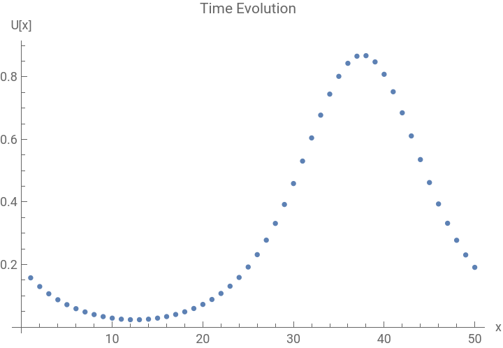
Since the advection equation represents the mass conservative law mathematically, we expect that the function U[x,t] (mass density of, say, pollutants in a moving fluid) is not smeared in time. However, due to the inherent dissipative feature of numerical methods, especially the FORCE scheme, the function is expected to be gradually smeared over time (one can check it by choosing a relatively large value of the cutoff, e.g., cutoff = 20, to avoid any local mesh refinement). On the other hand, if we choose a moderately low value for the cutoff, such as 0.1, we can see from the animation that the dissipation over time is somehow compensated by the adaptive mesh refinement, which is an outstanding result.
Potential connections to the Wolfram model and future work
Potential connections to the Wolfram model and future work
The Wolfram model is a powerful tool for generating abstract hypergraphs (a hypergraph is a generalization of a graph) [2]. The core of this model is the rules for rewriting collections of relations (between nodes). A very simple example of a rule is {{x,y}}{{x,z},{z,y}}. This rewriting rule basically creates a new node z between node x and y every time it applies. The following code is a simple graphical demonstration of how this model works with our simple rewriting rule:
RulePlot[ResourceFunction["WolframModel"][{{{x,y}}->{{x,z},{z,y}}}],VertexLabels->Automatic,"RulePartsAspectRatio"->0.5]
Out[]=
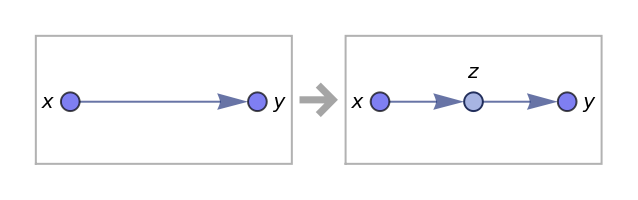
This simple example shows that the Wolfram model has the potential to be used as an adaptive mesh refiner in our code. However, particular care must be paid in employing the Wolfram model as in finite volume schemes, unlike finite difference ones, the graph nodes are not the computational nodes anymore. Indeed, they are the boundary nodes and the computational ones lie at the center of graph edges. A possible way to circumvent this issue for the 1D case could be imagining our initial uniformly-spaced grid is made of two superimposed identical but displaced grids; one for the computational nodes and one for the boundaries. However, keeping simultaneous track of the evolution of both graphs is challenging as it requires finding a dynamic relation between the rewriting rules. Another alternative to ease the situation is to think the boundary and computational nodes are, indeed, the nodes of one graph; we believe both approaches are feasible from a practical point of view. Possible extensions of this work would be generalizing this code to 2 or 3D cases and investigating the anti-dissipative nature of it, or re-writing the adaptive mesh refinement algorithm based on the Wolfram model and comparing the results with the present ones.
Keywords
Keywords
◼
Hyperbolic PDEs
◼
Advection Equation
◼
Finite Volume Method
◼
FORCE scheme
◼
Adaptive Mesh
◼
Limited Slope Rule
◼
Wolfram Model of Hypergraph of Rewriting Systems
Acknowledgment
Acknowledgment
I would like to express my special thanks of gratitude to my mentor, Mano Namuduri. This work would not be finished without her. I would also like to thank Xerxes D. Arsiwalla for his kind support and follow-ups. Last but not least, I want to thank Nik Murzin for his technical supports.
References
References
◼
[1] D. Vanzo, A. Siviglia, Finite Volume methods and Riemann Problem solvers, URL: https://ethz.ch/content/dam/ethz/special-interest/baug/ifu/env-fluid-mechanics-dam/documents/NumHyd/NumHyd_lectureNotes/Lecture_notes_FVM.pdf
◼
[2] S. Wolfram (2020), A Project to Find the Fundamental Theory of Physics, Wolfram Media Inc., URL: https://www.wolfram-media.com/products/a-project-to-find-the-fundamental-theory-of-physics.html