This code determines the reactor volume and operating temperature that minimize the total cost of achieving a target conversion in a continuous stirred-tank reactor (CSTR). The reaction follows first-order kinetics with an Arrhenius-type rate constant (k₀ = 1.2×10⁸ min⁻¹, activation energy Ea = 60,000 J/mol), and the goal is to process a feed flow rate of 5.0 L/min to a desired conversion of 95%. The cost function combines a capital cost proportional to reactor volume ($15/L) with a heating cost that penalizes deviations from ambient temperature (298 K), creating a genuine trade-off: smaller reactors need higher temperatures to hit the conversion target, but higher temperatures cost more to maintain.
The first solution method uses Mathematica’s built-in NMinimize function to solve the constrained optimization problem directly, subject to the CSTR design equation (which links volume, temperature, and conversion through the rate constant) and a temperature bound of 300–500 K. This approach converges to an optimal volume of 29.4982 L and an optimal temperature of 413.957 K, yielding a minimum cost of $1518.16 — serving as a benchmark solution against which pso method can be checked.
The second approach implements Particle Swarm Optimization (PSO), a population-based metaheuristic that mimics social behavior in swarms of bees. Rather than solving the constraint analytically, the design equation is folded into the fitness function as a penalty term (weighted by 10⁶) that punishes solutions violating the volume-temperature relationship. The psoOptimize function is built with standard PSO mechanics: particles with positions and velocities, personal-best and global-best tracking, inertia weight decay from 0.9 to 0.4 over iterations, and velocity clamping to prevent divergent search behavior.
Running the PSO optimizer with 30 particles over 8000 iterations shows the swarm’s loss steadily declining from over 1600 down to a plateau around 1518.2, closely tracking the NMinimize benchmark. The convergence log printed every 500 iterations reveals rapid early improvement followed by fine-tuning, with the loss essentially flatlining after iteration 3500 — a typical PSO convergence characteristic.
Finally, the notebook compares both methods directly: PSO’s global best position lands at volume ≈ 29.3997 L and temperature ≈ 414.039 K with a cost of $1518.2, remarkably close to NMinimize’s exact optimum of $1518.16.
A log-scale convergence plot visualizes the swarm’s cost trajectory, confirming that this heuristic, derivative-free approach can reliably reproduce the results of a dedicated numerical optimizer — a useful validation for applying PSO to problems where analytical or gradient-based methods will be difficult or impossible to implement.
ClearAll["Global`*"]
volumetric flow rate in L/min
q=5.0;
Desired conversion
X=0.95;
$/L coefficient for Reactor cost
CR=15;
$/K^2 Heating cost coefficient
CH=0.08;
Arrhenius Equation
k0=1.2*10^8;(*1/min*)Ea=60000;(*J/mol*)R=8.314;(*J/mol.K*)k[T_]:=k0Exp[-Ea/(RT)];
Design equation for CSTR
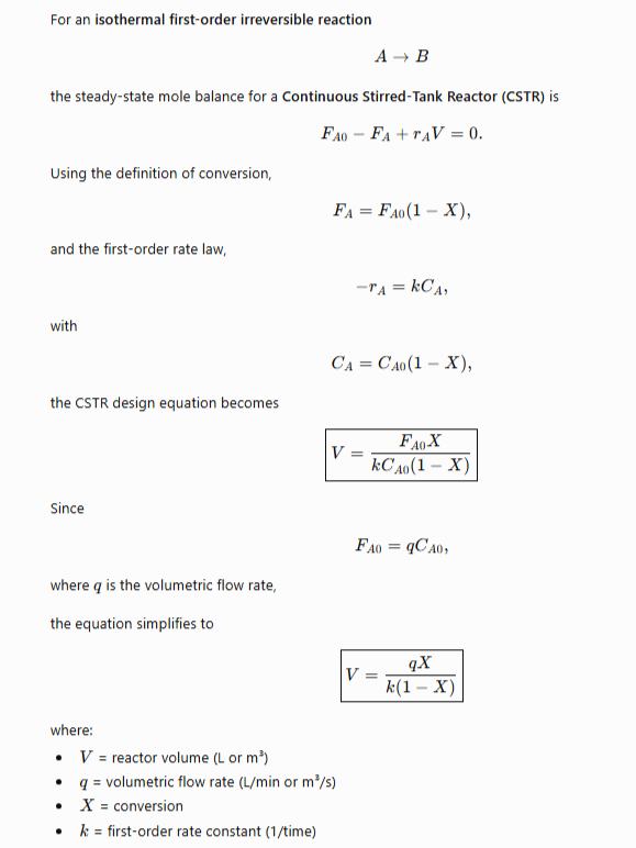
Method based on NMinimize
Method based on NMinimize
Objective Function
Cost[V_,T_]:=CRV+CH(T-298)^2;
Optimization
solution=NMinimize[{Cost[V,T],V==qX/(k[T](1-X)),300<=T<=500,V>=0},{V,T},AccuracyGoal->20,PrecisionGoal->20,Method->"DifferentialEvolution"]
Vopt=V/.Last[solution];Topt=T/.Last[solution];Costopt=First[solution];Print["Optimal Volume = ",Vopt," L"];Print["Optimal Temperature = ",Topt," K"];Print["Minimum Cost = $",Costopt];
Out[]=
{1518.2,{V29.3979,T414.04}}
Optimal Volume = 29.3979 L
Optimal Temperature = 414.04 K
Minimum Cost = $1518.2
PSO approach
In[]:=
Fitness[{V_,T_}]:=Cost[V,T]+10^6(V-qX/(k[T](1-X)))^2
SwarmDim=2;(*2Dproblem*)
Upper and lower bounds for the search domain
FitnessLB={0,300};FitnessUB={100,600};
PSO parameters
c1=1.42;c2=1.42;w=0.72984;
Clip each COLUMN of a matrix against its own scalar bound
clipMatrix[mat_,lbv_,ubv_]:=Transpose[MapThread[Clip[#1,{#2,#3}]&,{Transpose[mat],lbv,ubv}]];clampMatrix[mat_,vmaxv_]:=Transpose[MapThread[Clip[#1,{-#2,#2}]&,{Transpose[mat],vmaxv}]];
PSO Optimizer
psoOptimize[lossFunc_,dim_,lb_,ub_,nParticles_:30,nIter_:100,wMax_:0.9,wMin_:0.4,c1_:1.42,c2_:1.42,vClampFrac_:0.2]:=Module[{particles,velocities,pbest,pbestScore,gbest,gbestScore,convergence={},r1,r2,scores,gbestIdx,vmax,wIter},vmax=vClampFrac*(ub-lb);particles=Transpose@Table[RandomReal[{lb[[i]],ub[[i]]},nParticles],{i,dim}];velocities=ConstantArray[0.,{nParticles,dim}];pbest=particles;pbestScore=lossFunc/@particles;gbestIdx=First@Ordering[pbestScore,1];gbestScore=pbestScore[[gbestIdx]];gbest=pbest[[gbestIdx]];Do[wIter=wMax-(wMax-wMin)*(j-1)/(nIter-1);r1=RandomReal[1,{nParticles,dim}];r2=RandomReal[1,{nParticles,dim}];velocities=wIter*velocities+c1*r1*(pbest-particles)+c2*r2*(ConstantArray[gbest,nParticles]-particles);velocities=clampMatrix[velocities,vmax];particles+=velocities;particles=clipMatrix[particles,lb,ub];scores=lossFunc/@particles;pbest=MapThread[If[#3<#2,#1,#4]&,{particles,pbestScore,scores,pbest}];pbestScore=MapThread[Min,{pbestScore,scores}];gbestIdx=First@Ordering[pbestScore,1];If[pbestScore[[gbestIdx]]<gbestScore,gbestScore=pbestScore[[gbestIdx]];gbest=pbest[[gbestIdx]];];AppendTo[convergence,gbestScore];If[Mod[j,500]==0,Print["PSO Iter ",j," Loss = ",gbestScore]];,{j,nIter}];{gbest,gbestScore,convergence}];
PSO run
result=psoOptimize[Fitness,SwarmDim,FitnessLB,FitnessUB,100,8000];{gbest,gbestScore,convergence}=result;
PSO Iter 500 Loss = 1607.34
PSO Iter 1000 Loss = 1570.74
PSO Iter 1500 Loss = 1567.48
PSO Iter 2000 Loss = 1520.66
PSO Iter 2500 Loss = 1519.01
PSO Iter 3000 Loss = 1518.47
PSO Iter 3500 Loss = 1518.3
PSO Iter 4000 Loss = 1518.2
PSO Iter 4500 Loss = 1518.2
PSO Iter 5000 Loss = 1518.2
PSO Iter 5500 Loss = 1518.2
PSO Iter 6000 Loss = 1518.2
PSO Iter 6500 Loss = 1518.2
PSO Iter 7000 Loss = 1518.2
PSO Iter 7500 Loss = 1518.2
PSO Iter 8000 Loss = 1518.2
PSO result vs . NMinimize solution
PSO result vs . NMinimize solution
In[]:=
gbest
Out[]=
{29.3997,414.039}
In[]:=
gbestScore
Out[]=
1518.2
In[]:=
Print["Optimal Volume = ",Vopt," L"];Print["Optimal Temperature = ",Topt," K"];Print["Minimum Cost = $",Costopt];
Optimal Volume = 29.3979 L
Optimal Temperature = 414.04 K
Minimum Cost = $1518.2
PSO convergence plot
CITE THIS NOTEBOOK
CITE THIS NOTEBOOK
Optimal design of a CSTR reactor: balancing capital and energy costs via global optimization
by Housam Binous
Wolfram Community, STAFF PICKS, July 4, 2026
https://community.wolfram.com/groups/-/m/t/3744889
by Housam Binous
Wolfram Community, STAFF PICKS, July 4, 2026
https://community.wolfram.com/groups/-/m/t/3744889