CITE THIS NOTEBOOK: Studying Phase Transition in 2D Ising Model with Multiway Systems by Adiba Shaikh. Wolfram Community JAN 13 2023.
In this project, we study the ferromagnetic phase transition in the 2D Ising model. Using the 1D cellular automaton (CA) rules, we begin our analysis by finding the energy conserving rules for an arbitrary length of linear (1D) spin chain. Having the sample space of such evolution rules, we study the dynamical evolution of this system in terms of multiway graphs. Extending our analysis to 2D grid of spins for its multiway evolution under energy preserving rules, we set to explore the signatures of phase transition for a fixed energy of the system and varying spin densities (as effective temperature).
1. Introduction
1. Introduction
In statistical mechanics, Ising model is a model to study phase transition which consists of an array of spins aligned either up (+1) or down (-1) with nearest neighbour interaction. This model was developed by Lenz and studied by Ising (1920-25) in 1-dimensional system, where it was found to be no phase transition. The 2-dimensional version of this system of spins was studied by Onsager (1944) who proved that there is a phase transition occurring in such systems due to occurrence of spontaneous magnetization at low temperatures. The model is developed to study phase transitions in a system undergoing a change from ferromagnetic state (spin alignment) where the system exhibits non-zero net magnetization to demagnetized/paramagnetic state (random spin orientation) with no net magnetization, as the temperature is increased above its critical value ).
(
T
c
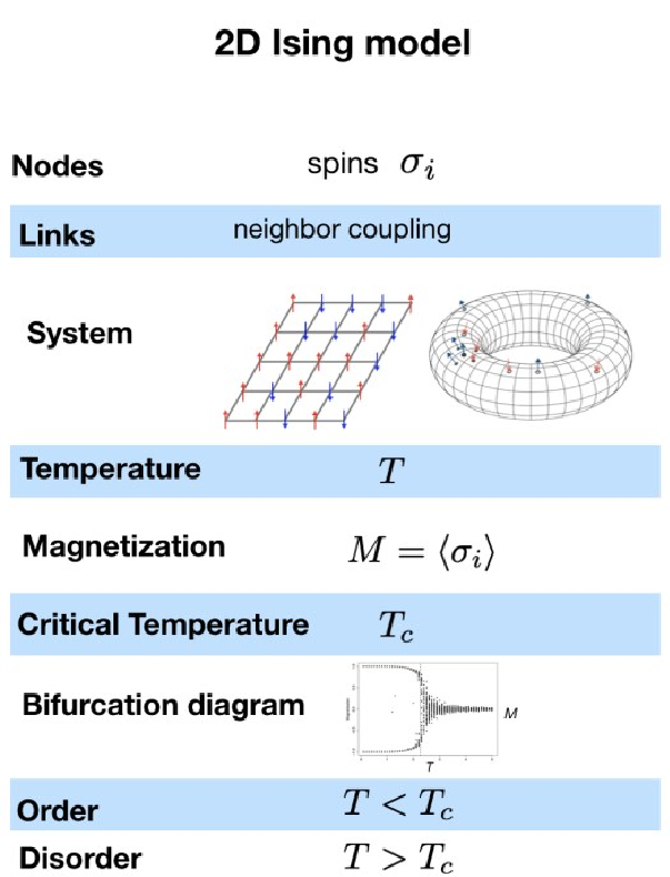
Phase transition occurs in systems which are unstable with respect to variation in thermodynamical parameters, e.g, ice-water-steam transition. The degree of order at a microscopic level that a system persists is quantified in terms of its order parameter. The variation of order parameter with change in a thermodynamical quantity from non-zero value to zero, is taken as an indication of the phase transition. E.g., in Ising model, magnetization or net number of up or down spins is taken as the order parameter.
Energy=-JMagnetization=
1
2
∑
ij
σ
i
σ
j
∑
i
σ
i
Cellular Automaton (CA) is a computational model for evolution of state where every step proceeds to next by application of a uniquely identified set of rules. A wide range of phenomena associated with dynamics from simple to complex system can be studied using CA. Such models are classical in a sense that given a seed (initial state) it has a definite path of its evolution. However, multiway systems [2] can be use to study the evolution of system in a probabilistic way to represent the different possible paths a system can evolve with time. In this work we studied an Ising model like system of spins in 1D chain and 2D grid in the absence of an external field. We identified the CA rules which preserve energy for successive evolutionary steps of spin states. Using such rules as a sample space for possible evolution of a system with a constant energy, we model its evolution on the multiway systems and look for the hints of phase transition.
For a system of the spin configuration, its magnetic energy corresponds to the sum of the pairwise taken spins. Here, for the spins at the edge we used cyclic or periodic boundary condition (last spin is paired with the first). The net magnetization of the system is the sum over all the spin orientations.
Energy and magnetization of the system with a particular spin configuration [1]:
In[]:=
spinEnergy[s_]:=(-1/2)*Total[sListConvolve[{{0,1,0},{0,1,0},{0,1,0}},s,2],2]spinMagnetization[s_]:=Total[s,2]
For a microcanonical ensemble, the temperature of the system can change, keeping its energy fixed. The magnetization of the system varies with temperature.
Magnetization as a function of inverse temperature (β = 1/T):
In[]:=
M[β_]:=Plot[{-M[β],M[β]},{β,0,Pi},AxesLabel->{"β","M"},Filling->Axis]
1/8
(1-)
-4
Sinh[2β]
Out[]=
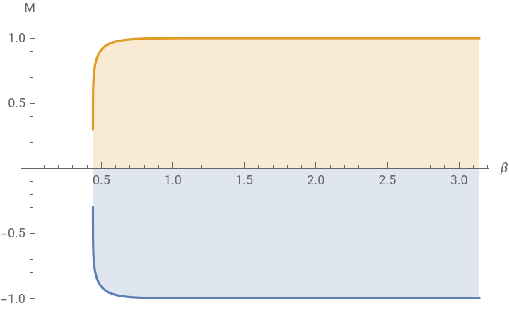
The spin system exhibits a net magnetization at large β (low T) which disappears at low β (high T) due to spontaneous symmetry breaking leading to a phase transition.
For a canonical ensemble, the change in magnetization of the system can be studied at different energies.
For a canonical ensemble, the change in magnetization of the system can be studied at different energies.
Magnetization (M) as a function of energy (E):
Manipulate[s=Tally[{spinEnergy[#],spinMagnetization[#]}&/@Tuples[{-1,1},{n,n}]];t=FlattenAt[s,Table[{x,1},{x,1,Length[s]}]];ListDensityPlot[t,FrameLabel->{Style["Energy",Bold,13],Style["Magnetization",Bold,14]},ColorFunction->"Rainbow"],{{n,4,Style["Spin grid size: ",13]},{2,3,4}},SaveDefinitions->True]
Out[]=

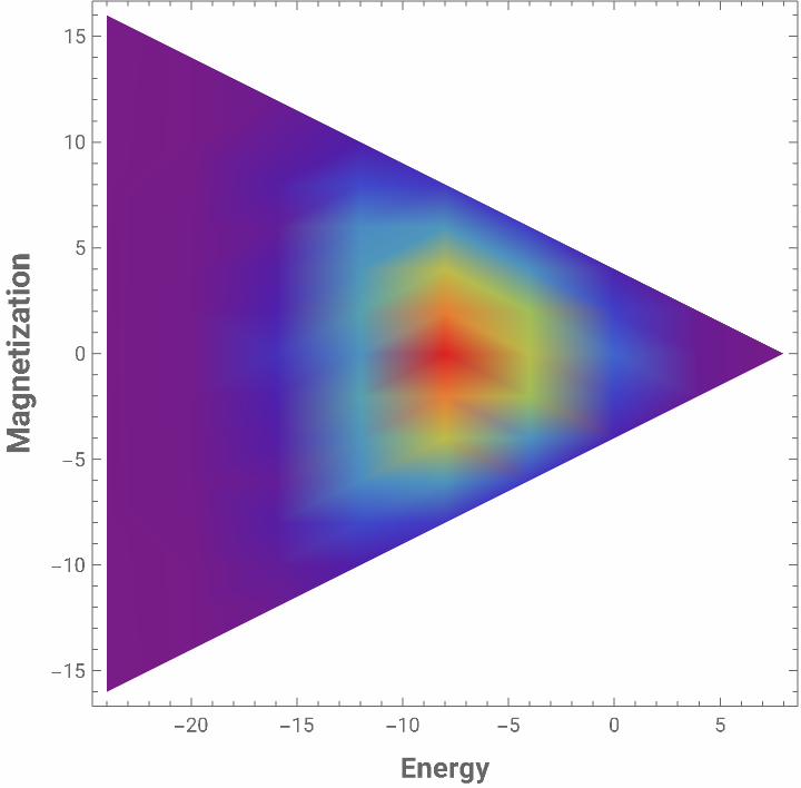
We see that at low energies, the density of states is small and fixed between +M or -M (non-ergodic). As the energy of the system is increased, large number of states get populated towards M=0, which results in vanishing of the net magnetization (ergodic) and results in a phase transition.
2. 1D Ising model
2. 1D Ising model
The 1D Ising model consists of a series of up and down spins arranged in a linear manner like a chain of spins. The interaction of any spin is only with the one to its left and to its right. The last or rightmost spin interacts with the first or leftmost spin, making a spin cycle. Here, we evolve the spin cycles under different 1-dimensional CA rules to find those that conserve energy.
2.1 Energy conserving CA rules for 1D spin chain:
2.1 Energy conserving CA rules for 1D spin chain:
Using the notation for up spin as (+1) and down spin as (-1), we first list out their possible combinations for any given number of spins. To reduce the complexity and evolution time, we take 3 spin cycle.
Possible spin cycle configurations for a given length of spin chain in 1D:
In[]:=
SpinConfig1D[s_]:=Tuples[{1,-1},s]SpinConfig1D[3]
Out[]=
{{1,1,1},{1,1,-1},{1,-1,1},{1,-1,-1},{-1,1,1},{-1,1,-1},{-1,-1,1},{-1,-1,-1}}
There are =8 possible configuration of 3 spins with each one having 2 states (up or down).
3
2
Visual representation of up (black/1) and down (white/-1) spins:
In[]:=
AssociationThread[SpinConfig1D[3],ArrayPlot[{#},Mesh->True]&/@(SpinConfig1D[3]/.{-1->0})]//Dataset
Out[]=
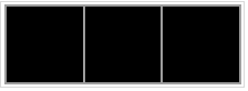
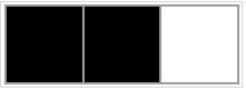
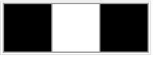
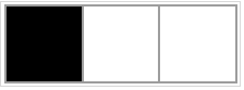
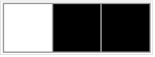
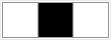
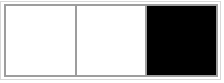

The energy of a spin cycle is the sum of all possible products of spin pairs, without duplication.
Spin cycle energy for an arbitrary length of spin chain in 1D:
The energies corresponding to all possible spin combinations for a given length of spin cycle can be found.
Possible energies of different spin cycles:
There are only two possible energies that this system of 8 states can have, with the degeneracy.
Energy corresponding to each of the spin configuration:
An alternate way to look this system as if each spin is only interacting to its nearest neighbour on its left and to its right. Hence, convolving the spin cycle with appropriate choice of interaction matrix should give them the same result as before.
An alternate expression for finding the spin energy configuration:
Association between spin cycles (grey cell) and their corresponding energies (white cells):
There are two states (all 3 up or all 3 down) having energy -3 and six states (1 or 2 up/down) spins with energy +1.
Energy values with their respective degeneracies:
We feed all 8 possible configurations of 3 spin cycle as the initial state of 256 1-dimensional CA and get their evolution after the first step to check for the change in energy. Note that the input to 2-color CA can be 1 or 0. Hence, we need to modify the down spin value (-1 -> 0) which later has been changed back to its original value (0 -> -1).
The output of 256 rules of 1D CA after first evolution step for a specific length of spin cycle:
We calculate the energy for the 8 outputs of each of the 256 CA rules.
Energies corresponding all possible outputs for a specific length of spin cycle:
Comparing the energy of each of the 8 states of 3 spin cycle after passing through the 256 CA rules with their initial energies, we can select those which gives the same final energy and filter those CA rules.
Filtering 1D CA rules with same energy before and after the evolution :
Total number of energy conserving 1D CA rules for 3-spins chain:
The number of CA rules conserved for 1D cycle of spins seems to be changing with the number of spins. We can find the variation of number of energy conserving CA with the length of spin cycle.
Function to find the total number of energy conserving CA rules for 1D spin chains of arbitrary length:
We check taking up to 10 spin configuration and the number of energy conserving rules asymptotically saturates to 34 for spin chain of length greater than or equal to 5.
Association between number of spins and the number of energy conserving CA rules :
The 34 1-dimensional CA rules giving energy conservation are:
2.2 Multiway systems of 1D spin chain:
2.2 Multiway systems of 1D spin chain:
In this section, we studied the evolution of the N-spin cycle under energy conserved 1D CA rules with multiway graphs [3]. Since, the number of conserved CA rules in the large number of spin limit turns out to be 34 as seen in the previous section. We restrict the evolution of spin chains over these set of rules. The dynamical evolution of spin states in the multiway system gives the probabilistic approach to study such spin systems.
Multiway system for possible evolution of the given initial state of 3-spin configuration over 3 evolutionary steps:
In above case, there are only 2 possible states, all up {1,1,1} and all down {-1,-1,-1} having the same energy -3. Hence, under energy conserving CA rules, the two states just make transition among each other. We can check for the remaining 6 states (having same energy +1) of the 3-spin cycle if there transition respects energy conservation.
Evolution of other states of 3-spin configuration (with energy -1) over 3 steps:
The 6 possible states - {{1,1,-1}, {1,-1,1}, {1,-1,1}, {1,-1,-1}, {-1,1,-1}, {-1,1,1}} having the same energy +1 make transition among themselves.
For a slightly larger number of spins, the multiway graphs seems to have a complex structure of evolution between energy conserving states.
For a slightly larger number of spins, the multiway graphs seems to have a complex structure of evolution between energy conserving states.
Multiway system for possible evolution of the given initial state of 5-spin configuration over 2 steps:
It would be interesting to see the evolution of states and their connectivity governed by various CA rules that conserve energy across different spin configuration.
Visualize the effect of spin density (effective temperature) change for energy preserving CA on a random state of large number of spins:
In the above visualization, each successive CA time evolution of spin chain is arranged below the previous one in a form of a 2D grid .
3. 2D Ising model
3. 2D Ising model
For the 2D Ising model, we have constructed a grid of NxN spins interacting with their nearest four neighbours (up, down, left, right). Each NxN matrix of spins can be constructed from the 1D chain of N-spins as rows and columns with periodic boundary condition applied to the edges. Similar to the 1D case, our goal is to find the CA rules that satisfy conservation of energy.
3.1 Energy conserving CA rules for 2D spin grid:
3.1 Energy conserving CA rules for 2D spin grid:
First we list all the possible different configurations of the two 1D spin chain of length 3 (simple choice) combined to form a 2D grid represented by 3x3 matrix.
Possible 2D spin cycle configurations from combining any two spin chain of equal length in 1D:
The energy of a spin grid is the sum of all possible products of spin pairs interacting along the four directions. The overall scaling down by factor of (1/2) is needed to account for double counting.
Energy of the NxN grid of spins in 2D:
Listing all possible energies of 2D spin grid, the system seems to be having degenerate states amongst its total 512 states.
Association between energies (grey cell) and their respective degeneracies (white cell) for 3x3 spin grid:
We observe that there is a unequal distribution of states across possible different energies of 2D system.
Energy values with their respective degeneracies:
All 512 possible configurations of 3x3 spin matrix are used as the initial state of 256 1-dimensional CA and they are evolved to check for their final state energy. Similar to the 1D case, the input to 2-color CA has been modified for down spin (-1 -> 0) which later has been changed back to its original value (0 -> -1).
The output of 256 rules of 1D CA after first evolution step for all possible 512 states of 2D spin:
We then proceed to calculate the energies of the 512 outputs using all of the 256 CA rules.
Energies corresponding all possible outputs for a specific size of spin grid:
Explicit values of energies and their degeneracy of total 512 states over going through one evolution step of 256 CA rules:
Previously found energies and corresponding degeneracy for the initial 512 states:
Comparison between the energy of each of the 512 initial states of 3x3 spin grid before and after passing through the 256 CA rules help us to find the energy preserving CA rules.
Filtering 1D CA rules with same energy before and after the evolution :
Total number of energy conserving 1D CA rules for 3x3 grid of spins:
We can compare the energy conserving CA rules found in the previous section for 1D spin chain with that of 2D spin grid to check for an overlap.
Note that we did not tried this exercise for different sizes of grid (4x4, 5x5, etc.) like in the 1D case for different length of spin chains in order to narrow down the asymptotic number of energy conserving CA rules in the limit of large 2D spin systems.
We will compare the energy conserving CA rules for 3 spin in 1D with 3x3 spins in 2D
Total number of energy conserving 1D CA rules for 3 spin cycle:
Intersection of energy conserving CA rules for 3 spin cycle (1D) to 3x3 spin grid (2D):
Complement of those energy conserving CA rules for 3 spin cycle (1D) which are absent for 3x3 spin grid (2D):
Complement of those energy conserving CA rules for 3x3 spin grid (2D) which are absent for 3 spin cycle (1D):
A null set indicates that:
1.) All the energy conserving rules for 2D grid of size 3x3 also preserves energy for 1D chain of length 3.
2.) The set of energy conserving rules for 2D grid of size 3x3 forms a subset of those for 1D chain of length 3.
It will remain further to investigate whether this property holds true for increasing number of spins in 1D and 2D and what is the saturation value of the number of energy preserving CA rules in 2D.
3.2 Multiway systems of 2D spin grid:
3.2 Multiway systems of 2D spin grid:
Once we narrow down the number of energy conserving CA rules (at least for 3x3 case), we studied the evolution of the 3x3-spin grid using the multiway graphs over the 24 energy conserving rules found in previous subsection. Here, we study the dynamical evolution of 2D spin states.
Multiway system for possible evolution of the given initial state of 3x3-spin configuration over 3 steps:
Let us check for the energy of any two states which are causally connected to see if they give same value:
Yes, indeed, we have a energy conserving multiway system here!
Evolution of another state of 3x3-spin configuration (with different energy) over 3 steps:
And yet again we see an another 3x3 states evolving along the energy conserving path.
The next step would be to connect such energy preserving dynamics of spin (possible microcanonical ensemble) to study phase transition in 2D Ising model. This serve as a motivation for our future studies along this line of work.
For now, it is worthy to explore a resource function IsingModelCA [4] which constructs the 2D grid of NxN spins with random initial spin state and evolve it under change of spin-coupling interaction strength considering it as a measure of the effective temperature.
Visualize the effect of spin density (effective temperature) as the system evolves to look for the signatures of phase transition:
Local clusters of spin alignment at low temperatures which disappears at high temperatures could be a hint of possible phase transition from ordered to disordered phase.
Concluding remarks
Concluding remarks
Keywords
Keywords
◼
Ising Model
◼
Phase Transition
◼
Cellular Automata
◼
Multiway Systems
Acknowledgment
Acknowledgment
I would like to acknowledge my mentors Jon Lederman and Tom Lee for their support and encouragement during the course of this project. I also would like to express my gratitude to Xerxes Arsiwalla for useful discussions and guidance, and the organizers for giving me this opportunity. Finally, I thank Stephen Wolfram for defining this interesting project for me.
References
References