Introduction
Introduction
This essay, I feel, can definitely be considered as belonging to the series that includes my last post, designed as an introduction to multivariable calculus; it follows along as what I called a ‘computational lecture’, being that I am hoping to teach a small topic assisted by the fantastic powers of the Wolfram Language.
The SIR model is certainly the most famous of all disease models, and is three years from turning a hundred. I find that it is a fantastic first step into mathematical modelling (and by extension, biological mathematics), as from here it is quite intuitive as to how we can expand models to deal with more complex ideas. The maths discussed here is, like last time, explained so that you shouldn’t even need a great grasp of calculus to understand what’s going on. The actual SIR model is relatively simple: so you will forgive me if I dwell a little on the theory behind it.
As a nota bene, the mathematics in this post is not overly difficult, but you may need to spend some time yourself looking at what’s going on. Like the last post, this might not be of interest to many but might help anyone new to this subject, or new to the Wolfram Language.
The SIR model is certainly the most famous of all disease models, and is three years from turning a hundred. I find that it is a fantastic first step into mathematical modelling (and by extension, biological mathematics), as from here it is quite intuitive as to how we can expand models to deal with more complex ideas. The maths discussed here is, like last time, explained so that you shouldn’t even need a great grasp of calculus to understand what’s going on. The actual SIR model is relatively simple: so you will forgive me if I dwell a little on the theory behind it.
As a nota bene, the mathematics in this post is not overly difficult, but you may need to spend some time yourself looking at what’s going on. Like the last post, this might not be of interest to many but might help anyone new to this subject, or new to the Wolfram Language.
A Literary Consideration of the SIR Model and its Limitations
A Literary Consideration of the SIR Model and its Limitations
SIR stands for Susceptible, Infectious and Removed (although some people may call the latter ‘recovered’). It considers the idea that all people in a population belong to either the S-group, I-group, or R-group (which is when they have either recovered and therefore are immune, or died). From there we can create a number of differential equations that allow us to predict infections and such from simple variables. You may see me refer to these groups as compartments, categories, etcetera - but officially the SIR model is compartmental.
Immediately, I hope you will note a major problem in this model: the idea that infected people are fully immune. As we have seen in the COVID-19 pandemic, it is completely possible to contract a disease multiple times, and this is in part due to the multiple strains that can arise, which circumvent the immune response from a previous strain’s infection.
Similarly, the model assumes infection is immediate: indeed, certain upon contact. There is a more advanced model that considers the ‘exposed’ group: the SEIR model. It should be quite obvious by the time we reach the end of this as to how we can change a simple model like this into one dealing with more complex ideas like that.
Two final points (but bear in mind these are not all the limitations); the model, put forth here, does not consider birth rates and natural deaths (nor does it give a number to how many potential deaths could be caused by a disease); it is also deterministic, rather than stochastic. If you are unfamiliar with these terms, a deterministic model is completely certain in variables such as how many people one person can infect. A stochastic model introduces elements of randomness which can provide a more accurate state of a natural system, being that the entirety of nature is inherently random.
Immediately, I hope you will note a major problem in this model: the idea that infected people are fully immune. As we have seen in the COVID-19 pandemic, it is completely possible to contract a disease multiple times, and this is in part due to the multiple strains that can arise, which circumvent the immune response from a previous strain’s infection.
Similarly, the model assumes infection is immediate: indeed, certain upon contact. There is a more advanced model that considers the ‘exposed’ group: the SEIR model. It should be quite obvious by the time we reach the end of this as to how we can change a simple model like this into one dealing with more complex ideas like that.
Two final points (but bear in mind these are not all the limitations); the model, put forth here, does not consider birth rates and natural deaths (nor does it give a number to how many potential deaths could be caused by a disease); it is also deterministic, rather than stochastic. If you are unfamiliar with these terms, a deterministic model is completely certain in variables such as how many people one person can infect. A stochastic model introduces elements of randomness which can provide a more accurate state of a natural system, being that the entirety of nature is inherently random.
The Mathematics (and Code) Behind It
The Mathematics (and Code) Behind It
Hopefully you are familiar with the idea of the derivative, which is most commonly seen in the form . This is mathematical shorthand for ‘the change in function y with respect to x’. Remember that the function itself will look something like f(x)=..., with x being the inputted value. Before we delve into how this works for the SIR model, we need to take a look at solving differential equations.If you have knowledge of calculus at A-level standard (or read my last post), you will have solved differential equations before. We do this all the time to find stationary points, because we solve the differential equation when it is equal to 0 (as that is when the gradient is 0). From there we can get the coordinates of those points. In the Wolfram Language, we can do this easily with the Solve function, for example:
y
x
Solve cos(x) = 0, with respect to x (where the graph of cos(x) crosses the x-axis).
Solve[Cos[x]==0,x]
Out[]=
x,x
Mathematica returns this in a nice form as it gives both solutions with the variable , where is an integer: in other words, giving an infinite number of solutions, as we would expect.
However differential equations can, and frequently do in applied mathematics, appear in a form containing both the derivative of a function, and the function itself. Take this: y’(x) + y(x) = x^2. To solve it, we need to find the function y(x) that can give us x^2 from the equation. Doing this by hand is relatively simple, but the Wolfram Language has a nice function:
c
1
c
1
However differential equations can, and frequently do in applied mathematics, appear in a form containing both the derivative of a function, and the function itself. Take this: y’(x) + y(x) = x^2. To solve it, we need to find the function y(x) that can give us x^2 from the equation. Doing this by hand is relatively simple, but the Wolfram Language has a nice function:
Find y(x) that satisfies the equation, where the function is y[x] and the variable is x.
DSolve[y'[x]+y[x]==x^2,y,x]
Out[]=
{{yFunction[{x},2-2x++]}}
2
x
-x
1
As you can see, the function fits perfectly. An important note here: this syntax is relevant to version 14.0. Please make sure that you check the updated documentation if you’ve upgraded.
DSolve is useful, but more importantly we have NDSolveValue, which gives us a numerical result (rather than symbolic), and allows us to easily plot it. The key idea with NDSolve is that we have to provide some data to the function, which allows us to actually graph the result. We also need to set the size of the Domain. Using the same equation from earlier:
DSolve is useful, but more importantly we have NDSolveValue, which gives us a numerical result (rather than symbolic), and allows us to easily plot it. The key idea with NDSolve is that we have to provide some data to the function, which allows us to actually graph the result. We also need to set the size of the Domain. Using the same equation from earlier:
Solving and plotting the equation for y(x), assuming y(0) = 10, and the domain is between 0 and 20.
sol=NDSolveValue[{y'[x]+y[x]==x^2,y[0]==10},y,{x,0,20}];Plot[sol[x],{x,0,20}]
Out[]=
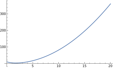
That assumption above is arbitrary, but it allows us to get a specific graph (rather than a general one, like we saw from DSolve earlier).Perhaps you’ve realised why we’ve been looking at all this calculus: when modelling diseases, we are fundamentally looking at the rates of change. This is because those rates are constantly changing - if more people are infected, there is a higher likelihood of a greater number people becoming infected the next day. Let me recall your mind to our three compartments of the SIR model: Susceptible, Infected, and Removed.These three are all going to change at different rates, so we need three different differential equations with respect to time: ,,. The total population is equal to the values of S, I and R summed, and is generally called N. Consider what happens after an outbreak: the number of Susceptible people decrease, and those infected move into the Infected compartment. At the same time, a number of people become immune at a different rate, into the Removed category. In other words: = -βSI = βSI-γI = λINote that the first differential equation (you may see this referred to as an ODE, or Ordinary Differential Equation, being that it only has one independent variable) represents the people being infected and leaving the Susceptible compartment. This is due to interactions between the Susceptible and Infectious groups, hence why it has two variables. The people who are entering the Removed group are doing that after a number of days, so it is only relevant to the Infectious people.Gamma, γ, is the rate of recovery, and therefore 1/γ is the infectious period. If the infectious period is 14 days, for example, gamma is 1/14. It’s worth noting here that people cannot die, and recover after a set period of time. Stochastics can help with the latter, and the former is even easier to implement - when we consider the code later, try and see how you might add it in.Beta, β, controls how often infection occurs between the Suscpetible and Infectious groups. It is often called the rate of infection: this is a misnomer. βI is the rate.Our model here can be simplified because the population is constant: once we know the number of people in the Susceptible and Infectious categories, we can simply subtract this from N (the population overall) to get the value of those recovered. This is worth considering but not worth it, because expanding the model is more complex from there.Here is an interesting idea; at the start of an outbreak, the infectious group is close to 0, so the S-group is approximately the entire population. Our second ODE can be written, factorising out the Infectious and replacing S with N: = I(βN-γ)Think about this logically, rather than in context. Given that Beta and Gamma are constants, if βN-γ < 0, the rate of change of I is decreasing. If it’s bigger than 0, the rate of change is increasing, and therefore we will see a positive gradient and increase in infections from Day 1. Scientifically, this is an epidemic. Otherwise the disease ‘dies out’. We’ll be able to see this in action later on. Now, βN-γ < 0 can be rearranged by adding γ to both sides and then dividing by it. We get (βN)/γ < 1. This is , also called the reproductive ratio or just the R value. You’ll probably have seen this in news articles and the like, particularly during the first year or two of the COVID-19 pandemic. If it is above 1 we see an epidemic. Note that means the R value at the start of the pandemic: how many people can one host infect in a population with no other (or very few) infected people. represents the R value later in an epidemic, and is therefore equal to (βS)/γ. In the real world, the R value is subject to all sorts influences, such as lock-downs.This is, essentially, all the mathematics needed for the SIR model, and all that remains is to actually program it. The code that follows should hopefully help to reinforce the ideas set out here, and show you how you can expand it.
S
t
I
t
R
t
S
t
I
t
R
t
I
t
R
0
R
0
R
t
Programming the SIR Model
Programming the SIR Model
Our first steps are to create our constants. We’ll begin with a population of 100,000 to see the general result. The R-value and gamma here are similar to those of the COVID-19 virus. Beta is calculated from the R-value, which is itself generally found from tracing backwards from hospitalisations and such. Below, only 1 person is infected.
Where there are 14 days to recovery, and the starting R value is 3.
In[]:=
R0=3;GAMMA=1/14;POPULATION=100000;BETA=R0*GAMMA/POPULATION;I0=1;
After that, we prepare our differential equations and get their numerical solutions. We know that at the start of the pandemic there are no Removed, and the number of people Susceptible is the total population - those infected. In other words, I[0] = 1 from above, R[0]=0, and S[0] = 9999, where the time is in days.
At each point in time the rate of change is dependent on the number of people in each compartment. The time range is between 0-150 days.
{susceptible,infectious,recovered}=NDSolveValue[{s'[t]==-BETA*s[t]*i[t],i'[t]==BETA*s[t]*i[t]-GAMMA*i[t],r'[t]==GAMMA*i[t],s[0]==POPULATION-I0,i[0]==I0,r[0]==0},{s,i,r},{t,0,150}]
Out[]=
InterpolatingFunction,InterpolatingFunction,InterpolatingFunction


This gives us three functions for each of S, I and R. From here, we can very easily plot the results (one of the reasons the Wolfram Language is so good for projects like this):
Plot[{susceptible[t],infectious[t],recovered[t]},{t,0,150},PlotStyle->{Dashing[Large],Dashing[Tiny],Dashing[Medium]},PlotLegends->{"Susceptible","Infectious","Removed"}]
Out[]=
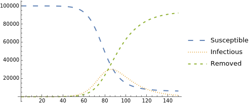
Et voilà, a fully functional disease model. What’s interesting here is that despite infections nearing 0 at the end, those susceptible plateau quite far above. This is an example of herd immunity, in which there are so many people who cannot contract the disease that, were you still susceptible, you would be very unlucky to get it yourself.
To extend ourselves a bit further, we can use the great ‘Manipulate’ function, that allows us to change certain variables.
To extend ourselves a bit further, we can use the great ‘Manipulate’ function, that allows us to change certain variables.
In[]:=
Manipulate[BETA=R0*GAMMA/POPULATION;{susceptible,infectious,recovered}=NDSolveValue[{s'[t]==-BETA*s[t]*i[t],i'[t]==BETA*s[t]*i[t]-GAMMA*i[t],r'[t]==GAMMA*i[t],s[0]==POPULATION-I0,i[0]==I0,r[0]==0},{s,i,r},{t,0,150}];Plot[{susceptible[t],infectious[t],recovered[t]},{t,0,150},PlotStyle->{Dashing[Large],Dashing[Tiny],Dashing[Medium]},PlotLegends->{"Susceptible","Infectious","Removed"}],{R0,2.5,10},{GAMMA,1/21,1},{POPULATION,1000,10000000},{I0,1,1000}]
Where we can manipulate R0, Gamma, the population and number of infected between the values specified above.
Out[]=
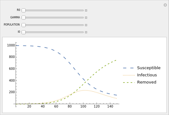
The code above is exceedingly messy, but it does the job. If you’re interested I would recommend running it yourself, as you can see some interesting patterns emerging.
This is, effectively, it. As I mentioned earlier, I don’t want to delve any further in because hopefully now you can see how everything works and be able to expand it yourself.
This is, effectively, it. As I mentioned earlier, I don’t want to delve any further in because hopefully now you can see how everything works and be able to expand it yourself.
Conclusion
Conclusion
Let’s recap quickly: we have looked at the idea of solving ODEs in the Wolfram Language, both symbolically and numerically; 2-dimensional plots of results; the SIR model itself; and creating an interactive model for further research. I hope you found this interesting, until the next time!
P.S. To expand your knowledge/recap check out the Further Reading below!
P.S. To expand your knowledge/recap check out the Further Reading below!
Further Reading
Further Reading
◼
Good for a quick recap and extending the model: https://www.wolfram.com/broadcast/video.php?v=3669
◼
A fantastic course for the Wolfram Language and disease models, going into great depth: https://www.wolfram.com/wolfram-u/courses/data-science/building-applying-epidemiological-models-dat931/
◼
A brilliant book for a complete introduction to Mathematical Biology: https://sheffield.pressbooks.pub/introducingmathematicalbiology/
CITE THIS NOTEBOOK
CITE THIS NOTEBOOK
A beginner's guide to the SIR model
by Theo Vine
Wolfram Community, STAFF PICKS, January 3, 2025
https://community.wolfram.com/groups/-/m/t/3350139
by Theo Vine
Wolfram Community, STAFF PICKS, January 3, 2025
https://community.wolfram.com/groups/-/m/t/3350139