Wolfram Cloud Document

A brief tutorial on energy landscape analysis of ecological communities
by Kenta Suzuki
RIKEN BRC Integrated Bioresource Information Division

In Suzuki et al. (2021), we used Mathematica to implement a new approach for analysis of ecological communities, which we called energy landscape analysis. In this article, we explain how to use the package and provide concrete examples to help illustrate the concepts.

1. Introduction

Energy landscape analysis is a systematic method for analyzing an energy landscape represented as a weighted network (Fig. 1). In the energy landscape, the nodes of the network represent unique community compositions, and the links represent the transition paths between them. The community composition is described as a binary vector that represents the presence (1) and absence (0) of a species, and the links connect all nodes that differ only in the presence or absence of one species. The nodes are weighted by their energies, and the difference in energy level drives the direction of transitions in community composition. Transitions from high-energy states to low-energy states occur more frequently than vice versa. The energy is assigned by a pairwise maximum entropy model or its extension with an external force (environmental effect) term. The parameters of the model are estimated by matching the expected probability of community compositions given by the model to empirical probabilities calculated from the observed data.
(For details of the method, see Suzuki et al. 2021.)

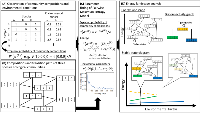
Figure 1. Illustrative explanation of our approach. (A) we assume that the dataset to be analyzed includes occurrence of species in local communities sampled from multiple targets (e.g., sites, hosts) and/or timepoints, with possibly accompanying values representing local environmental condition (environmental factors). (B) the state space of community compositions is formally defined as a graph. (C) observational data is used to fit parameters in a pairwise maximum entropy model. (D) the fitted pairwise maximum entropy model specifies an energy landscape which is a network with nodes representing community states and links representing transitions between community compositions. Energy landscape analysis acknowledges the stable states and tipping points. The disconnectivity graph summarizes the hierarchical relationships between the stable states and tipping points, and its change over environmental conditions can be described as a stable state diagram.

2. Materials

The package ela and datasets for this tutorial (datasets.zip) is available from GitHub:
https://github.com/kecosz/ela

datasets.zip contains two csv files. abundance_table.csv is a table of species abundance for each sample (a set of observations obtained from the same environment, such as lakes and marshes, plant root, animal skin, etc.). Although abundance may reflect counts of taxa other than species, we use “species” in this article for the sake of simplicity. sample_metadata.csv is a table of the environmental conditions of the observation sites where the samples were obtained, and contains the values of some environmental factors. Here, the values are assumed to be numerical, but labels corresponding to ordinal scales can be used after converting them into numerical values.

3. Energy landscape analysis

3.1 Data preparation

The first step is to load the package and data. In the following, it is assumed that the package has been downloaded to “D:/ela” and the contents in datasets.zip has been extracted to the datasets folder under the ela folder:

SetDirectory["D:\\ela"];(*setaccordingtoyourenvironment*)Needs["ela`"]baseabtable=Import["datasets\\abundance_table.csv","CSV"];basemetadata=Import["datasets\\sample_metadata.csv","CSV"];

The following is a part of the abundance table:

TableForm[Take[#,8]&/@Take[baseabtable,8]]

	species.1	species.2	species.3	species.4	species.5	species.6	species.7
sample.1	2384	0	1313	8218	0	3529	0
sample.2	10343	0	2201	6814	0	2887	0
sample.3	4473	0	614	2046	4455	3429	0
sample.4	8786	0	5517	328	0	15	0
sample.5	10640	0	2321	6652	0	2642	0
sample.6	0	0	165	7794	1697	3816	0
sample.7	8801	0	2204	4853	0	5526	0

The following is a part of the metadata:

TableForm[Take[basemetadata,8]]

	factor.1	factor.2
sample.1	-0.92	2.79692
sample.2	0.34	2.14701
sample.3	-0.92	1.60611
sample.4	-0.24	0.584765
sample.5	0.4	1.73161
sample.6	-0.82	2.95972
sample.7	0.36	0.0778733

In each case, the rows contain values of the same sample. This format must be followed.

In order to generate the “objects” to be used in the energy landscape analysis, the loaded data are preprocessed by
the following Formatting function:

{ocmatrix,abmatrix,fctmatrix,samplelabel,specieslabel,factorlabel}=Formatting[baseabtable,basemetadata,0,{0.05,0.05,0.95}];

Processed 256 samples.Relative abundance threshold = 0.05,Occurrence threshold (lower) = 0.05,Occurrence threshold (upper) = 0.95.Selected 16 out of 16 species.

The first and second arguments are the frequency table and metadata loaded above. The third argument is whether or not to normalize the abundances within the sample; 0 for without normalization, 1 for normalization. The fourth argument is a vector of threshold values, and it contains a threshold for converting abundance to presence/absence status, a lower bound of the count of presence (1) status (any species with a ratio of presence status less than this value is excluded) and an upper bound of the ratio of presence status (any species with a ratio of presence status greater than this value is excluded).Formatting returns six objects. Here, we assigned the following variable names to them:1. ocmatrix: matrix of the presence(1)/absence(0) status of each species in each sample2. abmatrix: matrix of the abundance of each species before converting to the presence/absence status3. fctmatrix: matrix of the environmental condition (a set of environmental factors) for each sample4. samplelabel: list of sample names5. specieslabel: list of species names6. factorlabel: list of environmental factorsocmatrix and abmatrix are S×N matrices where S represents the number of species and N represents the number of samples, and fctmatrix is an M×N matrix where M represents the number of environmental factors. Each row of ocmatrix represents a community composition, which is independently represented as a binary vector with length S.

3.2 Parameter fitting

First, the analysis is performed without considering the differences in environmental conditions among the samples. For this purpose, the following pairwise maximum entropy model is used:

(k)

-E(

(k)

)

ZE(

(k)

)=-

∑

i=1

(k)

∑

j=1

∑

i=1,i≠j

(k)

2Z=

-1

∑

k=0

-E(

)

Here, h is a vector of length S, and J is a S×N matrix. The superscript k means that σ(k) is the kth among all possible community compositions (binary vectors).

By executing the following SimpleSA function, parameter estimation is performed using ocmatrix as the training data:

SeedRandom[2];(*Thisshouldberemoved.*)AbsoluteTiming[{hest,jest,updt}=SimpleSA[ocmatrix,10^-5];]

{3.4761,Null}

The first argument should always be the presence/absence matrix, and the second argument is a threshold to determine the convergence of the parameters and stop the calculation. SimpleSA updates the parameters in several steps and automatically stops when it judges that the parameters have converged. (In order to simplify the explanation, the estimation is performed only once, but multiple trials can be performed in parallel using ParallelTable, and the mean value of the estimated parameters can be used.)

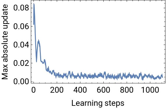
The first and second return values of SimpleSA (hest, jest) are the estimates of h and J, respectively. The third return value (updt) is the largest absolute value of the parameter updates at each step. This sequence of numbers can be used to check the convergence of the parameters. If convergence is not achieved, the second argument of SimpleSA has to be smaller. This can be checked visually as follows:

ListPlot[updt,JoinedTrue,PlotRangeAll,FrameTrue,FrameLabel{"Learning steps","Max absolute update"},FrameStyleDirective[14,Black]]

3.3 Analysis and visualization of energy landscapes

The energy landscape analysis is performed by passing the estimated h and J to the function ELA:

AbsoluteTiming[ela=ELA[hest,jest];]{stablestates,ssenergy,tippingpoints,tpenergy}=ela;

{14.712,Null}

ELA returns four objects, which we assigned the following variable names:1. stablestates: list of composition IDs of the stable states2. ssenergy: energy of the above stable states3. tippingpoints: list of composition IDs of the community composition that is the tipping point between two stable states4. tpenergy: energy of the above tipping points

A stable state is a community composition that has lower energy than all the community compositions to which it is directly connected. When one or more stable states are found, they are considered to be representative of the ecological community of interest. Composition ID is obtained by converting the binary vector of a community composition into a decimal number. The composition IDs and the binary vectors of community compositions can be mutually converted as follows:

stablestatess=Length[ocmatrix[[1]]];bin=CIntegerDigits[#,s]&/@stablestatesFromDigits[#,2]&/@bin

Below is part of the tabular form of the composition ID of stable states, their energies and presence/absence status:

A tipping point is the community composition with the lowest energy among the energy barrier between two stable states. tippingpoints and tpenergy are in matrix form:

The positions of the elements of the above matrix correspond to the positions of community IDs in stablestates. For example, the integers in the first row and second column of tippingpoints (52428) is the composition ID of the tipping point between two stable states 19660 and 38092. The element of tpenergy is the energy of the community composition at the corresponding position.

3.4 Basin of attraction

Another important structure in understanding the energy landscape is the basin of attraction. When we choose a certain community composition and follow links where the energy decreases the most, we finally reach a stable state. A basin of attraction is a set of compositions that reach the same stable state, and can be labeled by the composition ID of the stable state. The size of a basin of attraction, i.e., the number of community compositions it contains, is an important indicator of the prevalence of stable states.

When a pair of community IDs of any community composition and its energy, and the estimates of h and J are given, the following Bi function returns a pair of a composition ID of stable state and its energy:

Each of the observed community compositions is always included in one of the basins of attraction (or is a stable state itself).
The following functions plot the observed community compositions on a two-dimensional plane using PCA and color-code them according to the basin of attraction to which they belong. The observed community compositions belonged to two major basins of attraction:

3.5 Disconnectivity graph

A disconnectivity graph provides a summary of the structure of an energy landscape. To draw a disconnectivity graph, first, pass the output of ELA (ela) to the function GraphObj, which returns a drawing object of a disconnectivity graph. Then, pass the drawing object to the DisconnectivityGraph function:

The tip of each branch is labeled with the composition ID of the stable state, and its position represents the energy of the stable state. (The composition IDs are subscripted with C to emphasize that they represent the community composition.) The pie chart is a visualization of the binary vector representing the community composition, where white and black represents presence and absence of species, respectively. In the joint parts of the branches, the composition IDs of the tipping points are shown. When there are two or more stable states at the end of a branch, there can be more than
one tipping point with the opposite branch. In such a case, the one with the lowest energy becomes the actual tipping point. Results of the example shown here suggest that the system has five stable states, two of which have deep basins of attraction.

3.6 Pruning

In some cases, an energy landscape contains stable states with very shallow basins of attraction. If there are many such stable states, the structure of the energy landscape becomes noisy. Since the chance that the community composition stays in such a stable state is considered to be short, the effect of omitting shallow basins of attraction and including them as part of a deeper basin is small.

ELPruning prunes stable states whose energy barrier (energy difference between a tipping point and the stable state) is shallower than rprn*100% compared to that of the stable state having the maximum height of energy barrier among all stable states in the energy landscape of interest. The pruned stable states and their basins of attraction are to be considered as part of the deeper basins to which they belong.

The first return value of ELPruning is the same as ELA. Therefore, we can use it to draw the Disconnectivity graph. In the result, only the two deepest basins of attraction are remained:

The second return value of ELPruning is the substitution rule for the stable state:

This indicates which stable state has been integrated with the stable states after pruning. This substitution rule can be used, for example, to modify the results of PCA shown earlier. The community compositions were found to be divided into two categories: 1) compositions belonging to a major basin of attraction, and 2) compositions belonging to a mino basin of attraction:

3.7 Analysis of interspecific relationships

The estimated parameters (jest) can be used to analyze the relationships among species. The following simple function takes the return value of ELA (the first return value in the case of ELPruning) as an argument, and outputs a network where links connecting species appearing in at least in one stable state based on their positive (blue) or negative (red) interactions. Each species is plotted on a two-dimensional plane based on the characteristics of their interactions. The example below suggests that the groups of species {2,7,12,16} and {1,8} or {4,6,14} are mutually exclusive. However, the presence of species 3 may facilitate the coexistence of the two groups of species, {2,7,12,16} and {1,8}.

4. Energy landscape analysis along with environmental gradients

Environmental conditions affect whether or not a species occurs in a habitat, and consequently affect the process of community assembly. In the following section, we explain the energy landscape analysis considering the influence of environmental conditions.

4.1 Data preparation and parameter estimation

First, load the package and data, and then preprocess it. This part is the same as 3:

Next, the environment factors are rescaled. Here, each environmental factor is transformed into a range with minimum 0 and maximum 1. To do this, just pass fctmatrix, the matrix of environmental factors for each sample, to the function FctRescale:

The first return value is the rescaled environment factor. The second return value is the original maximum and minimum value of each environmental factor and can be used to restore the rescaled values to their original scale.

The energy of each community composition considering the influence of environmental factors is estimated by the following extended maximum entropy model:

In addition to the first and second term, which are common to the pairwise maximum entropy model, a term encompassing the environmental response of each species is added. Here, g is an M×S matrix, where S is the number of species and M is the number of environmental factors.

Estimates of h, J, and g (hest, jest, gest) are obtained by executing the following function (reimplemented the algorithm in Chap.3 of Clark 2015):

Again, it is better to parallelize and take the average of the parameter estimates to get more stable results. From the fourth return value, we can see the convergence of the parameters:

4.2 Energy landscape along with changes in environmental factors

To obtain the energy landscape reflecting change in environmental factors, the function GradELA is used.
This function requires five arguments, which are prepared as follows: First, the estimates of h, j, and g should be combined together.

Next, the reference environmental condition must be specified. In the following analysis, one environmental factor is varied in the range of 0 to 1 (note that the values are rescaled), and the other factors are fixed to the reference. The reference may be set arbitrarily, or it may be the mean or median of each factor. Here, we use the median as the reference.

In addition, the number of energy landscapes in the range of 0-1 must be specified. If the number of steps is larger, the change of the energy landscape can be tracked more smoothly, but the computational complexity is also higher.

The fourth argument is the level of pruning.

The fifth argument specifies which environment factor is to be changed. In the following example, we set 1 as the argument thus the first environment factor is changed. Now we can run GradELA:

As the first return value of GradELA, steps environmental conditions used to compute the energy landscape are given. Each of them consists of M environmental factors. It can be confirmed that only the specified environmental factor (here, the first one) is changing:

The original scale of environmental factors can be restored as follows:

The second return value of GradELA is the result of the ELA run for the above steps, pruned at the specified level. It can be confirmed that each of them is the return value of ELA, i.e., consists of the composition IDs of the stable states, the energy of the stable states, the composition IDs of the tipping points, and the energy of the tipping points.

The third return value of GradELA is the drawing object of DisconnectivityGraph for each environmental condition. Thus, when one of these objects is passed, DisconectivityGraph draws the disconnectivity graph:

When these three return values are passed together, the function SSDobj generates a drawing object of a stable state diagram. SSDiagram uses this to draw a stable state diagram. (The environmental conditions can be either rescaled (genv) or the original scale (rgenv). In the following example, the original scale is used.)

The solid line represents the range of environmental condition in which stable states exist, and they are labeled with the composition ID of stable states. The dashed line represents the energy of the tipping points. (If the labels overlap and are difficult to see, just double-click on them to adjust their position.) Results of the above example suggest that the system has three branches of stable states starting from C59852, C38092, and C58001, with C59852 disappearing in the early stages, C38092 changing to C46476 and C46468, and C58001 changing to C58001 at the end. For the two branches that remain until the end, it was found that the branch of C58001 loses relative stability with environmental change.

The following figure shows the actual diagram of the community composition of this system. Looking at the correspondence with the stable state diagram, we can see that the number of stable states and the changes in the composition are captured, although the accuracy is rather coarse. (The vertical axis is the first component of PC because the energy is not defined for the actual community compositions.)

文献
1. Suzuki, K., Nakaoka, S., Fukuda, S., & Masuya, H. (2021).
Energy landscape analysis elucidates the multistability of ecological communities across environmental gradients. Ecological Monographs.
https://esajournals.onlinelibrary.wiley.com/doi/abs/10.1002/ecm.1469
2. Harris, D. J. (2015). Multi-Process Statistical Modeling of Species’ Joint Distributions. University of California, Davis.
https://figshare.com/articles/thesis/Multi_Process_Statistical _Modeling _of _Species _Joint _Distributions/3114226/1