PedalCurveCircumference::usage="References:https://e.math.cornell.edu>people;Personal.";
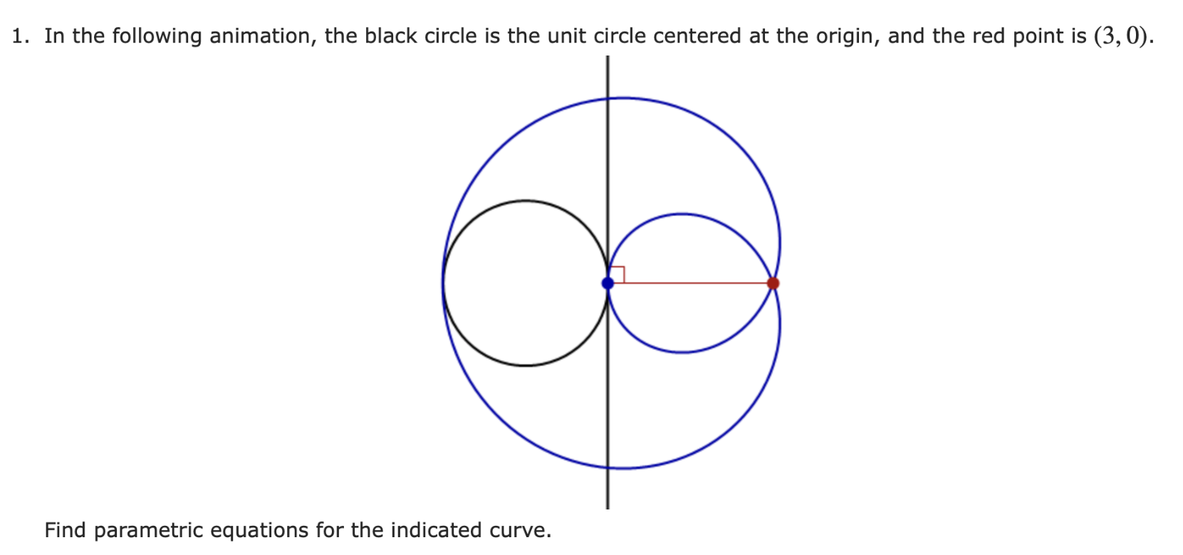
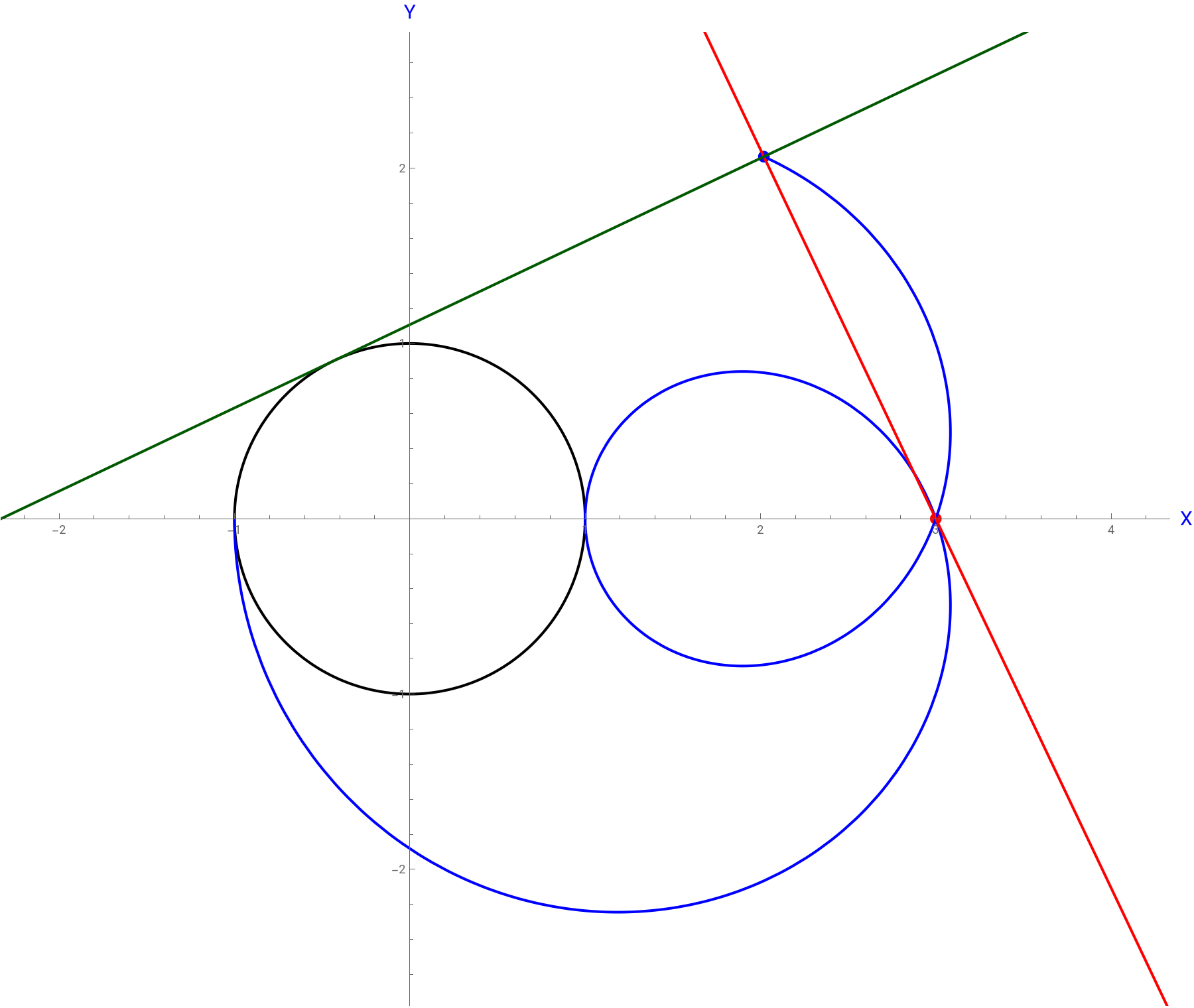
Development to obtain the parametric equations of the cardioid, which is the pedal curve of the circumference:
In[]:=
ζ[t_]:={Cos[t],Sin[t]};=ζ[t]+ζ'[t]//FullSimplify
ζ
P
ζ'[t].({3,0}-ζ[t])
2
Norm[ζ'[t]]
Out[]=
Cos[t]++,+
3
2
Sin[t]
2
Abs[Cos[t]]
2
Abs[Sin[t]]
(+-3Cos[t])Sin[t]
2
Abs[Cos[t]]
2
Abs[Sin[t]]
2
Abs[Cos[t]]
2
Abs[Sin[t]]
Cos[t]++,+;[t_]:={Cos[t]+3,(1-3Cos[t])Sin[t]};
3
2
Sin[t]
2
Abs[Cos[t]]
2
Abs[Sin[t]]
(+-3Cos[t])Sin[t]
2
Abs[Cos[t]]
2
Abs[Sin[t]]
2
Abs[Cos[t]]
2
Abs[Sin[t]]
ζ
P
2
Sin[t]
Animation:
In[]:=
SwatchLegend[{Black,Blue,DarkGreen,Red},{"Circumference","Pedal curve (cardioid)","Tangent line to the circumference","Orthogonal line to the tangent line and the point {3, 0}"}]Manipulate[ζ[t_]:={Cos[t],Sin[t]};[t_]:={Cos[t]+3,(1-3Cos[t])Sin[t]};Show[ParametricPlot[ζ[t],{t,0,2π},PlotStyle{Black,Thick}],Graphics[{Blue,PointSize[0.01],Point[[k1]]}],Graphics[{Red,PointSize[0.01],Point[{3,0}]}],ParametricPlot[[t],{t,-π,k1},PlotStyle{Blue,Thick},PerformanceGoal->"Quality"],Graphics[{Red,Thick,InfiniteLine[{{3,0},[k1]}]}],Graphics[{DarkGreen,Thick,InfiniteLine[{ζ[k1],[k1]}]}],AxesLabel->(Style[#,15,Blue]&/@{"X","Y"}),AxesOrigin{0,0},AxesTrue,AspectRatioAutomatic,PlotRange{{-2,4},{-2.5,2.5}},ImageSize900],{k1,-π+0.00001,π,0.00001},SaveDefinitionsTrue,ControlPlacementTop]
ζ
P
2
Sin[t]
ζ
P
ζ
P
ζ
P
ζ
P
Out[]=


Out[]=