This notebook numerically locates and classifies all stationary points of Himmelblau’s test function defined by:
f(x1,x2) = (x1^2+x2-11)^2+(x1+x2^2-7)^2
using Gray Wolf Optimization (GWO) launched from many random initial swarms/seeds. The resulting candidate points are collected into a stationary points table, then deduplicated (via a Norm[#1-#2] < edgeDedupTol tolerance test) into a final set called allninestationaryPts — confirming there are exactly nine stationary points. Each point is then classified (minimum, maximum, or saddle) by evaluating the Hessian matrix and its eigenvalues at that point (positive definite → minimum, negative definite → maximum, mixed signs → saddle), and the results are tabulated alongside the function value f(x1,x2) at each point.
Why exactly 9 stationary points?
Setting the gradient to zero gives two equations:
4x1 (x1^2+x2-11) + 2 (x1+x2^2-7)=0
2 (x1^2+x2-11) + 4 x2 (x1+x2^2-7)=0
Each of these is a cubic (degree-3) plane curve in (x1, x_2) — the leading terms 4x1^3 and 4x2^3 confirm the degree. Bézout’s theorem states that two plane algebraic curves of degrees m and n, with no common component, intersect in at most mxn points (counted with multiplicity, over the complex projective plane). Here, m=n=3, so the theorem bounds the number of stationary points at 3x3 = 9. For Himmelblau’s function this bound is achieved exactly, with all 9 intersection points real and finite: 4 local minima (the famous equal-valued global minima, f=0), 4 saddle points, and 1 local maximum — which is precisely what the PSO search and Hessian classification in this notebook recover numerically.
As an independent check on the swarm search, the notebook also runs FindMinimum directly — with no GWO involved — from a large table of scattered initial guesses (via Table and Parallelize), each time minimizing the squared-gradient-norm loss used to define the stationary points. Since FindMinimum is a purely local, gradient-based solver, every run converges only to whichever critical point lies within its own basin of attraction, so sweeping enough initial points and collecting the distinct limits should recover the same nine stationary points that GWO found. Agreement between the two independent methods — one metaheuristic and population-based, the other deterministic and local — gives confidence that GWO neither missed a stationary point nor converged to a spurious one
f(x1,x2) = (x1^2+x2-11)^2+(x1+x2^2-7)^2
using Gray Wolf Optimization (GWO) launched from many random initial swarms/seeds. The resulting candidate points are collected into a stationary points table, then deduplicated (via a Norm[#1-#2] < edgeDedupTol tolerance test) into a final set called allninestationaryPts — confirming there are exactly nine stationary points. Each point is then classified (minimum, maximum, or saddle) by evaluating the Hessian matrix and its eigenvalues at that point (positive definite → minimum, negative definite → maximum, mixed signs → saddle), and the results are tabulated alongside the function value f(x1,x2) at each point.
Why exactly 9 stationary points?
Setting the gradient to zero gives two equations:
4x1 (x1^2+x2-11) + 2 (x1+x2^2-7)=0
2 (x1^2+x2-11) + 4 x2 (x1+x2^2-7)=0
Each of these is a cubic (degree-3) plane curve in (x1, x_2) — the leading terms 4x1^3 and 4x2^3 confirm the degree. Bézout’s theorem states that two plane algebraic curves of degrees m and n, with no common component, intersect in at most mxn points (counted with multiplicity, over the complex projective plane). Here, m=n=3, so the theorem bounds the number of stationary points at 3x3 = 9. For Himmelblau’s function this bound is achieved exactly, with all 9 intersection points real and finite: 4 local minima (the famous equal-valued global minima, f=0), 4 saddle points, and 1 local maximum — which is precisely what the PSO search and Hessian classification in this notebook recover numerically.
As an independent check on the swarm search, the notebook also runs FindMinimum directly — with no GWO involved — from a large table of scattered initial guesses (via Table and Parallelize), each time minimizing the squared-gradient-norm loss used to define the stationary points. Since FindMinimum is a purely local, gradient-based solver, every run converges only to whichever critical point lies within its own basin of attraction, so sweeping enough initial points and collecting the distinct limits should recover the same nine stationary points that GWO found. Agreement between the two independent methods — one metaheuristic and population-based, the other deterministic and local — gives confidence that GWO neither missed a stationary point nor converged to a spurious one
Note that the code would likely run properly if one changes GWO function with any other appropriate function for a different metaheuristic algorithm such as
Genetic Algorithm (GA)
Particle Swarm Optimization (PSO)
Simulated Annealing (SA)
Differential Evolution (DE)
Ant Colony Optimization (ACO)
Artificial Bee Colony (ABC)
Whale Optimization Algorithm (WOA)
Firefly Algorithm (FA)
Cuckoo Search (CS)
Tabu Search
Harmony Search (HS)
Particle Swarm Optimization (PSO)
Simulated Annealing (SA)
Differential Evolution (DE)
Ant Colony Optimization (ACO)
Artificial Bee Colony (ABC)
Whale Optimization Algorithm (WOA)
Firefly Algorithm (FA)
Cuckoo Search (CS)
Tabu Search
Harmony Search (HS)
In[]:=
Classify each converged point via the Hessian eigenvalues
classify[{x_,y_}]:=Module[{eig},eig=Eigenvalues[hessf[x,y]];Which[Max[Abs[eig]]>1*^-4&&Min[eig]>0,"minimum",Max[Abs[eig]]>1*^-4&&Max[eig]<0,"maximum",Min[eig]<0&&Max[eig]>0,"saddle"]];
Finding all critical points via PSO by minimizing ||grad f||^2
Himmelblau function: f(x1,x2) = (x1^2+x2-11)^2+(x1+x2^2-7)^2
Himmelblau function: f(x1,x2) = (x1^2+x2-11)^2+(x1+x2^2-7)^2
ClearAll[f,loss,gradf,hessf];
Define the Himmelblau function
f[x1_,x2_]:=(x1^2+x2-11)^2+(x1+x2^2-7)^2
vars={x,y};
Gradient:{∂f/∂x,∂f/∂y}
gradf[x_,y_]:=Evaluate@D[f[x,y],{vars}]
Hessian using Outer
hessf[x_,y_]:=Evaluate@Outer[D[f[x,y],{#1,1},{#2,1}]&,vars,vars]
In[]:=
gradf[x,y]
Out[]=
{4x(-11++y)+2(-7+x+),2(-11++y)+4y(-7+x+)}
2
x
2
y
2
x
2
y
In[]:=
hessf[x,y]//MatrixForm
Out[]//MatrixForm=
2+8 2 x 2 x | 4x+4y |
4x+4y | 2+8 2 y 2 y |
Objective PSO will minimize: squared norm of the gradient
loss[{x_,y_}]:=Total[gradf[x,y]^2];
In[]:=
its=500;
Run several independent swarms (different random seeds) so we’re likely to land on all critical points
results=Table[GWO[loss,2,{-7,7},30,1000,seed],{seed,1,its}]
In[]:=
Print["Run gbest (x,y) ||grad||^2 classification"];Do[With[{pt=results[[k,1]],val=results[[k,2]]},Print[k," ",NumberForm[pt,{6,4}]," ",ScientificForm[val,3]," ",classify[pt]]],{k,Length[results]}];
Run gbest (x,y) ||grad||^2 classification
In[]:=
stationarypoints=Table[results[[k]][[1]],{k,1,its}];
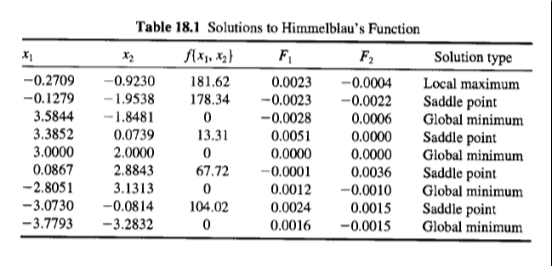
Removing duplicates yields only 9 stationary points in agreement with Bezout theorem and Table 18.1 of Ref . 1
In[]:=
edgeDedupTol=7*^-2;
In[]:=
allninestationaryPts=DeleteDuplicates[stationarypoints,Norm[#1-#2]<edgeDedupTol&]
Out[]=
{{3.38511,0.0736629},{-0.127904,-1.95372},{-0.270774,-0.922881},{-2.80763,3.13436},{-3.78229,-3.2888},{-3.07074,-0.0767912},{0.0865394,2.88431},{3.00054,1.99937},{3.58487,-1.84671}}
In[]:=
Length@allninestationaryPts
Out[]=
9
In[]:=
Join[{{Style["x1",Darker@Red],Style["x2",Darker@Red],Style["f(x1,x2)",Darker@Red],Style["solution type",Darker@Red]}},Table[{allninestationaryPts[[i]][[1]],allninestationaryPts[[i]][[2]],f[allninestationaryPts[[i]][[1]],allninestationaryPts[[i]][[2]]]//Chop,classify[{allninestationaryPts[[i]][[1]],allninestationaryPts[[i]][[2]]}]},{i,1,Length@allninestationaryPts}]]//TableForm
Out[]//TableForm=
x1 | x2 | f(x1,x2) | solution type |
3.38511 | 0.0736629 | 13.3119 | saddle |
-0.127904 | -1.95372 | 178.337 | saddle |
-0.270774 | -0.922881 | 181.617 | maximum |
-2.80763 | 3.13436 | 0.000568696 | minimum |
-3.78229 | -3.2888 | 0.00143459 | minimum |
-3.07074 | -0.0767912 | 104.015 | saddle |
0.0865394 | 2.88431 | 67.7191 | saddle |
3.00054 | 1.99937 | 0.0000107123 | minimum |
3.58487 | -1.84671 | 0.0000440267 | minimum |
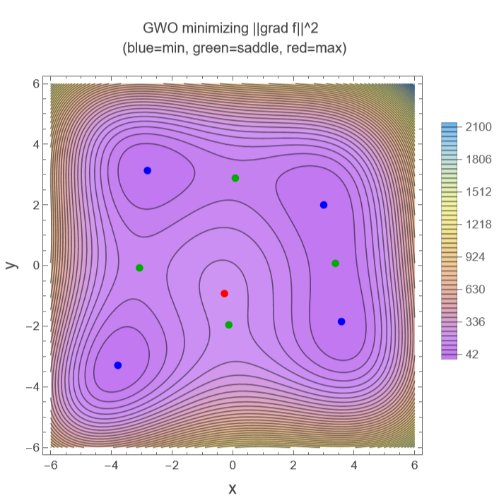
Contour plot of f with critical points displayed in red (maximum), green (saddle) and blue (minimum)
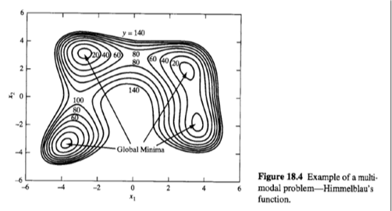
results in agreement with Fig. 18.4 of Ref. 1
results in agreement with Fig. 18.4 of Ref. 1
pts=allninestationaryPts[[All]];labels=classify/@pts;colorFor["minimum"]=Blue;colorFor["maximum"]=Red;colorFor["saddle"]=Darker[Green];plot=ContourPlotf[x,y],{x,-6.0,6.0},{y,-6.0,6.0},
Out[]=
Let us try a different strategy using FindMinimum with 1000 random initial guess taken in [-14,14]x[-14,14]
In[]:=
init=RandomReal[{-1,1},{1000,2}]*ConstantArray[14,1000]
In[]:=
LaunchKernels[]
Out[]=
KernelObject

In[]:=
sol=Parallelize@Table[{x,y}/.FindMinimum[loss[{x,y}],{x,init[[i]][[1]]},{y,init[[i]][[2]]}][[2]],{i,1,Length@init}]
In[]:=
sol2=DeleteDuplicates[sol,Norm[#1-#2]<edgeDedupTol&]
Out[]=
{{-0.127961,-1.95371},{-2.80512,3.13131},{-3.77931,-3.28319},{3.,2.},{3.58443,-1.84813},{-3.07303,-0.081353},{-0.270845,-0.923039},{0.0866775,2.88425},{3.38515,0.0738519}}
In[]:=
Length@sol2
Out[]=
9
Contour plot of f with critical points displayed in red (maximum), green (saddle) and blue (minimum)
results in agreement with Fig. 18.4 of Ref. 1
results in agreement with Fig. 18.4 of Ref. 1
pts=sol2[[All]];labels=classify/@pts;colorFor["minimum"]=Blue;colorFor["maximum"]=Red;colorFor["saddle"]=Darker[Green];plot=ContourPlotf[x,y],{x,-6.0,6.0},{y,-6.0,6.0},
CITE THIS NOTEBOOK
CITE THIS NOTEBOOK
Determining extrema of the Himmelblau function via Gray Wolf optimization and FindMinimum
by Housam Binous
Wolfram Community, STAFF PICKS, August 9, 2026
https://community.wolfram.com/groups/-/m/t/3775819
by Housam Binous
Wolfram Community, STAFF PICKS, August 9, 2026
https://community.wolfram.com/groups/-/m/t/3775819