ORIGINAL ARTICLE: A. Von-Held Soares, H. Binous, F. C. Peixoto, and A. Bellagi, Solving boundary value problems in heterogeneous catalysis with orthogonal collocation and arc-length continuation, Comput. Appl. Eng. Educ. (2023), e22701.
DOI: https://doi.org/10.1002/cae.22701
DOI: https://doi.org/10.1002/cae.22701
Article Abstract: An important part of the education of chemical engineers involves the design and assessment of heterogeneous catalytic reactions. They pose fundamental phenomena and constitute invaluable industrial processes. Progressing in this field, especially in graduate-level courses, entails solving nonlinear differential equations systems, which can only be achieved by using efficient and reliable numerical techniques. In this work, we solve nonisothermal one-dimensional reaction-diffusion BVP considering convection in the boundary conditions, by applying orthogonal collocation and arc-length continuation. Particularly, we predict the effectiveness factor as a function of the Thiele modulus for the main three particle geometries: plane slab, cylinder, and sphere. For chemical engineering students, such problems are at the zenith of the discipline, and the results of such calculations can elucidate basic and advanced concepts of mass and heat transfer as well as chemical reaction engineering. Both Chebyshev and shifted Legendre polynomials were used to transform the boundary value problem into a set of algebraic nonlinear equations. In addition, we also compare our findings against the available analytic solutions whenever possible. Codes in Scilab, Matlab®, and Mathematica© were developed for the solution of such problems and are available in the Supporting Information. There are two possible approaches to compute effectiveness factors: (a) integration as per definition versus (b) differentiation and nonlinear system. It is demonstrable that software performance is dependent on the approach, and that the differentiation approach yields better results.
Here, we solve nonisothermal one-dimensional reaction-diffusion Boundary Value Problem (BVP) considering convection in the boundary conditions, by applying orthogonal collocation and arc-length continuation. Particularly, we predict the effectiveness factor as a function of the Thiele modulus for spherical particle.
For chemical engineering students, such problems are at the zenith of the discipline, and the results of such calculations can elucidate basic and advanced concepts of mass and heat transfer as well as chemical reaction engineering.
Chebyshev polynomials were used to transform the boundary value problem into a set of algebraic nonlinear equations.
In addition, we also compare our findings against the solution given in Ref. 1.
There are two possible approaches to compute effectiveness factors: (a) integration as per definition versus (b) differentiation and nonlinear system.
We show in Ref. 2 that software performance is dependent on the approach, and that the differentiation approach yields better results.
In[]:=
(*TWENTYONECOLOCATIONPOINTS*)Np=20;y[i_]:=Cos[iPi/Np]//N;
In[]:=
(*DERIVATIVEMATRIX*)d[0,0]=(2Np^2+1)/6//N;d[Np,Np]=-(2Np^2+1)/6//N;d[i_,i_]:=-y[i]/(2(1-y[i]^2))//N;d[j_,k_]:=If[j!=k&&k!=0&&k!=Np&&j!=0&&j!=Np,(-1)^(j+k)/(y[j]-y[k])]//N;d[Np,0]=-1/2(-1)^Np;d[0,Np]=1/2(-1)^Np;d[j_,0]:=If[j!=Np&&j!=0,-1/2(-1)^j/(1-y[j])];d[j_,Np]:=If[j!=Np&&j!=0,1/2(-1)^(j+Np)/(1+y[j])];d[0,j_]:=If[j!=Np&&j!=0,2(-1)^j/(1-y[j])];d[Np,j_]:=If[j!=Np&&j!=0,-2(-1)^(j+Np)/(1+y[j])];A=Table[d[i,j]//N,{i,0,Np},{j,0,Np}];B=A.A;
In[]:=
(*SYSTEMOFEQUATIONS*)sys=Flatten[{Table[(4B.Table[x1[i][s],{i,1,Np+1}])[[i]]+2/((y[i-1]+1)/2)(2A.Table[x1[i][s],{i,1,Np+1}])[[i]]==p[s]^2Exp[g(1-1/x2[i][s])]x1[i][s],{i,2,Np}],Table[(4B.Table[x2[i][s],{i,1,Np+1}])[[i]]+2/((y[i-1]+1)/2)(2A.Table[x2[i][s],{i,1,Np+1}])[[i]]==-bp[s]^2Exp[g(1-1/x2[i][s])]x1[i][s],{i,2,Np}],(2A.Table[x1[i][s],{i,1,Np+1}])[[Np+1]]==0,(2A.Table[x2[i][s],{i,1,Np+1}])[[Np+1]]==0,(2A.Table[x1[i][s],{i,1,Np+1}])[[1]]==Sh(1-x1[1][s]),(2A.Table[x2[i][s],{i,1,Np+1}])[[1]]==Nu(1-x2[1][s]),Sum[x1[i]'[s]^2+x2[i]'[s]^2,{i,1,Np+1}]+p'[s]^2==1,Table[(2A.Table[ef[i][s],{i,1,Np+1}])[[i]]==3((y[i-1]+1)/2)^2Exp[g(1-1/x2[i][s])]x1[i][s],{i,1,Np}],ef[Np+1][s]==0}];
In[]:=
(*PARAMETERS*)Sh=100;Nu=18;g=15;b=1.0;
In[]:=
(*INITIALCONDITIONS*)init=Join[Flatten[Table[{{x1[j][0]==0.5},{x2[j][0]==1.1},{ef[j][0]==1.1}},{j,1,Np+1}]],{p[0]==0.01}];
In[]:=
SYS=Flatten[Join[sys,init]];
In[]:=
Length[SYS]
Out[]=
128
In[]:=
(*UNKNOWNS*)unk=Flatten[Join[Table[{x1[i][s],x2[i][s],ef[i][s]},{i,1,Np+1}],{p[s]}]];
In[]:=
Length[unk]
Out[]=
64
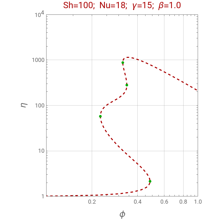
Let us compute and plot the effectiveness factor (dashed red line) as well as the four turning points (indicated by the green dots).
As one can see, there can be up to five steady-states for particular values of the Thiele modulus (of which only three are stable steady-states).
As one can see, there can be up to five steady-states for particular values of the Thiele modulus (of which only three are stable steady-states).
In[]:=
(*SOLUTIONOFTHEDIFFERENTIALALGEBRAICSYSTEMOFEQUATIONS,64EQUATIONS/64INITIALCONDITIONS/64UNKNWONS*)sol=Quiet@Reap@NDSolve[Flatten[Join[sys,init,{WhenEvent[p'[s]==0,Sow[{s}]]}]],unk,{s,-10^-3,10^3},AccuracyGoal->5];
In[]:=
(*locioftheturningpointsareobtainedusingthecommandWhenEvent*)tnpoints=Flatten@sol[[2]]
Out[]=
{1.27744,5.51286,9.81041,14.1726}
In[]:=
(*EFFECTIVENESSFACTOR*)EFTABLEsphere1=Table[Flatten[{p[s],ef[1][s]}/.sol[[1]]],{s,1000,0.001,-0.1}];
In[]:=
(*PLOTTINGTHEEFFECTIVENESSVERSUSTHETHIELEMODULUS*)p1=ListLogLogPlot[EFTABLEsphere1,PlotStyle->{Dashed,Darker@Red},Joined->True,Frame->True,GridLines->Automatic,PlotRange->{{0.1,1},{1,10^4}}];
Show[p1,Graphics[{PointSize[0.0175],Darker@Green,Table[Point[{Log[p[s]],Log[ef[1][s]]}]/.sol[[1]]/.s->tnpoints[[i]],{i,1,4}]}],ImageSize->350{1,1},AspectRatio->1.2,FrameLabel->{Style["ϕ",14],Style["η",14]},PlotLabel->Style["Sh=100; Nu=18; γ=15; β=1.0",Darker@Red,14]]
Out[]=
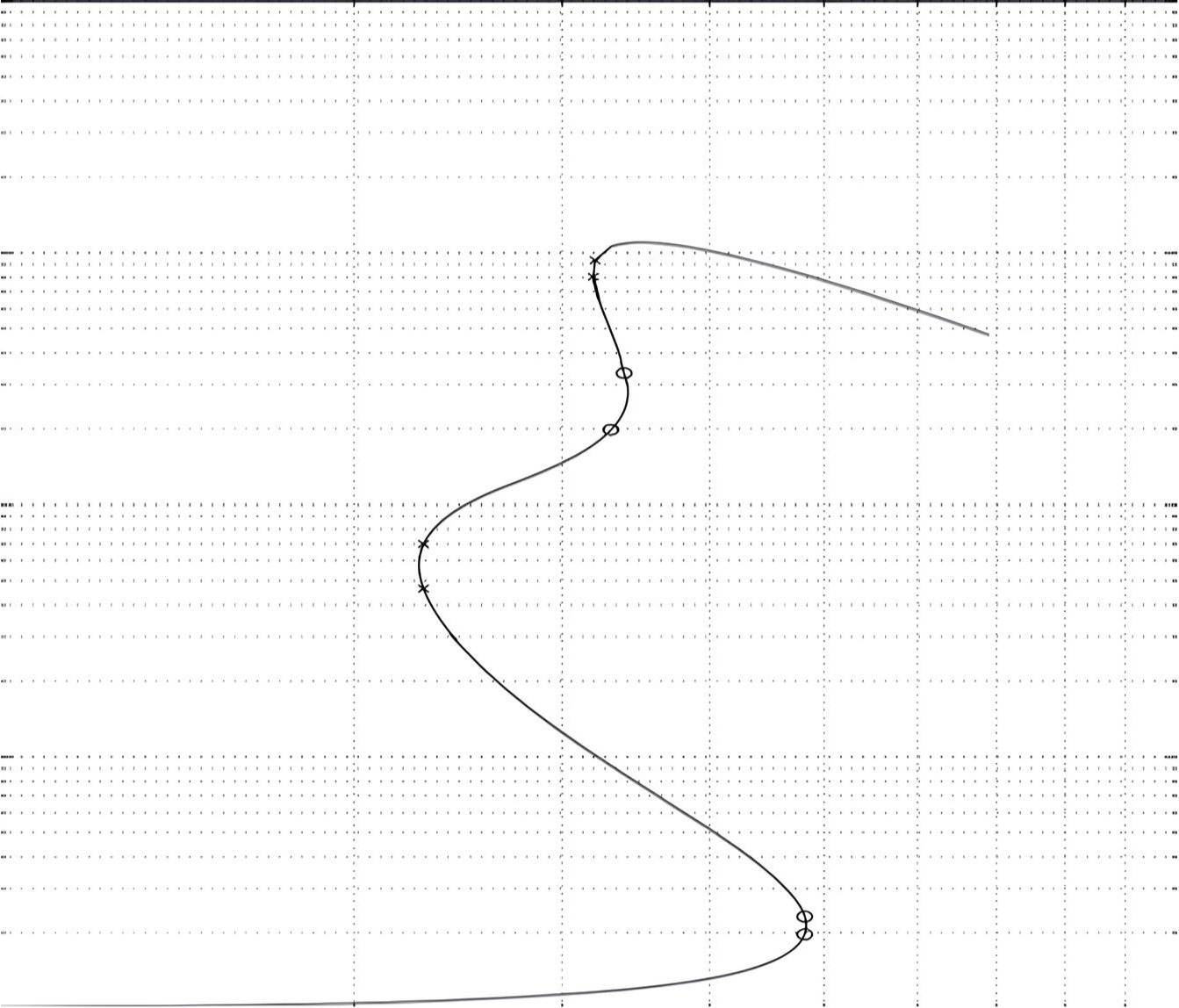
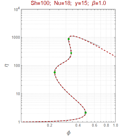
Let us compare our calculated effectiveness factor (dashed red line) with its counterpart (solid black line) given in Ref . 2.
As one can see agreement between both data is excellent.
As one can see agreement between both data is excellent.
IMG=
;(*Figure5-26page318copiedfromRef.1*)
In[]:=
Show[ListLogLogPlot[EFTABLEsphere1,PlotStyle->{Dashed,Darker@Red},Joined->True,Frame->True,GridLines->Automatic,PlotRange->{{0.1,1},{1,10^4}},ImageSize{350,350},AspectRatio->1.2,Prolog{Raster[ImageData[IMG,DataReversedTrue],{Scaled[{0.0,0.0}],Scaled[{1,1}]}]}],Graphics[{PointSize[0.0175],Darker@Green,Table[Point[{Log[p[s]],Log[ef[1][s]]}]/.sol[[1]]/.s->tnpoints[[i]],{i,1,4}]}],FrameLabel->{Style["ϕ",14],Style["η",14]},PlotLabel->Style["Sh=100; Nu=18; γ=15; β=1.0",Darker@Red,14]]
References
References
◼
[1] S. S. E. Elnashaie and F. Uhlig, Numerical techniques for chemical and biological engineers using MATLAB(R)—a simple bifurcation approach, Springer, New York, 2007. https://doi.org/10.1007/978-0-387-68167-2
◼
[2] A. Von-Held Soares, H. Binous, F. C. Peixoto, and A. Bellagi, Solving boundary value problems in heterogeneous catalysis with orthogonal collocation and arc-length continuation, Comput. Appl. Eng. Educ. (2023), e22701. https://doi.org/10.1002/cae.22701
CITE THIS NOTEBOOK
CITE THIS NOTEBOOK
Non-Isothermal Effectiveness Factor using Chebyshev Orthogonal Collocation and Arc-Length Continuation
by Housam Binous, André Von-Held Soares, Fernando Cunha Peixoto, and Ahmed Bellagi
Wolfram Community, STAFF PICKS, January 18, 2024
https://community.wolfram.com/groups/-/m/t/3105404
by Housam Binous, André Von-Held Soares, Fernando Cunha Peixoto, and Ahmed Bellagi
Wolfram Community, STAFF PICKS, January 18, 2024
https://community.wolfram.com/groups/-/m/t/3105404