The Liouville-space (vectorization) formulation turns the Markovian master equation into a single linear ODE, converting the Lindblad generator into a matrix acting on the vectorized density operator. This representation unifies state propagation, steady states, spectral decay/oscillation rates, two-time correlators, long-time asymptotics, and more. The complex Schur decomposition is the key numerical tool within the vectorized approach. Together, vectorization and Schur provide a compact, scalable, and numerically robust framework for modeling time-independent Lindblad evolution. In this short computational essay, I briefly review the vectorization formulation and the application of Schur decomposition to the dynamics of open quantum systems governed by the Lindblad equation.
I’d like to remind Mathematica users that scenarios we discussed here are fully supported under the hood by the design and structure of the Wolfram Quantum Framework. Here, for clarity and elaboration, we will delve into the vectorization formulation together with the application of Schur decomposition for the time evolution of open quantum systems, independent from Wolfram quantum framework. If any question or suggestion, you can reach out to us at quantum AT wolfram.com or leave a comment here.
Vectorize a square matrix:
In[]:=
vectorize[a_]:=Flatten[Transpose[a]]
Out[]=


One example for a 3x3 matrix:
In[]:=
Witha=Arraya.,{3,3},MatrixForm[a]->MatrixForm[vectorize[a]]
Out[]=
a.[1,1] | a.[1,2] | a.[1,3] |
a.[2,1] | a.[2,2] | a.[2,3] |
a.[3,1] | a.[3,2] | a.[3,3] |
a.[1,1] |
a.[2,1] |
a.[3,1] |
a.[1,2] |
a.[2,2] |
a.[3,2] |
a.[1,3] |
a.[2,3] |
a.[3,3] |
Check for a specific dimension:
vec[A.ρ]=(I⊗A).vec[ρ]
In[]:=
Module{dim,a,r},dim=5;a=Arraya.,{dim,dim};r=Arrayr.,{dim,dim};KroneckerProduct[IdentityMatrix[dim],a].vectorize[r]==vectorize[a.r]
Out[]=
True
Check for a specific dimension:
vec[ρ.A]=(⊗I).vec[ρ]
T
A
In[]:=
Module{dim,a,r},dim=5;a=Arraya.,{dim,dim};r=Arrayr.,{dim,dim};KroneckerProduct[Transpose[a],IdentityMatrix[dim]].vectorize[r]==vectorize[r.a]
Out[]=
True
Check for a specific dimension:
Tr[A]=vec[I].vec[A]
In[]:=
Module{dim,a},dim=3;a=Arraya.,{dim,dim};vectorize[IdentityMatrix[dim]].vectorize[a]==Tr[a]
Out[]=
True
Check for a specific dimension:
Tr[A.B]=vec[].vec[B]
T
A
In[]:=
Module{dim,a,b},dim=7;a=Arraya.,{dim,dim};b=Arrayb.,{dim,dim};Tr[a.b]==vectorize[Transpose[a]].vectorize[b]//Expand
Out[]=
True
Check for a specific dimension:
vec[A.X.B]=(⊗A).vec[X]
T
B
In[]:=
Module{dim,a,x,b},dim=3;a=Arraya.,{dim,dim};x=Arrayx.,{dim,dim};b=Arrayb.,{dim,dim};vectorize[a.x.b]==KroneckerProduct[Transpose[b],a].vectorize[x]//Expand
Out[]=
True
Lindblad equation which determines the evolution of the density matrix ρ is given by:
ℒ[ρ]=-[H,ρ]+.ρ.-,ρ
∑
k
L
k
†
L
k
1
2
†
L
k
L
k
In[]:=
ℒ[r_,h_,l_]:=-Commutator[h,r,Dot]+Sumlk.r.ConjugateTranspose[lk]-Anticommutator[ConjugateTranspose[lk].lk,r,Dot],{lk,l}
1
2
Vectorized Lindblad equation: =-(I⊗H-⊗I)+⊗-I⊗-⊗I and thus .vec[ρ]=vec[ℒ[ρ]]
ℒ
vec
T
H
∑
k
*
L
k
L
k
1
2
†
L
k
L
k
1
2
T
L
k
L
k
ℒ
vec
In[]:=
ℒvec[h_,l_]:=Module{n=Length[h],iden},iden=IdentityMatrix[n];-(KroneckerProduct[iden,h]-KroneckerProduct[Transpose[h],iden])+SumKroneckerProduct[Conjugate@lk,lk]-KroneckerProduct[iden,ConjugateTranspose[lk].lk]-KroneckerProduct[Transpose[lk].Conjugate[lk],iden],{lk,l}
1
2
1
2
Note in the above code, I used Commutator and Anticommutator that are new functions introduced in version 14.3 of Mathematica. If you have older versions, please replace those terms with the exact form of commutation or anticommutation.
Check .vec[ρ]=vec[ℒ[ρ]] for a specific dimension and given number of Lindblad operators:
ℒ
vec
In[]:=
Module{dim,numOfLindbladOperators,r,h,l},dim=3;numOfLindbladOperators=7;r=Arrayr.,{dim,dim};h=Arrayh.,{dim,dim};l=Array[#,{dim,dim}]&/@TableUniqueL.,{i,numOfLindbladOperators};vectorize[ℒ[r,h,l]]==ℒvec[h,l].vectorize[r]//Expand
Out[]=
True
Since and the time evolution is trace-preserving, then one needs .
Check that for a specific dimension and given number of Lindblad operators:
Tr[ρ]=vec[I].vec[ρ]
vec[I].ℒvec=0
Check that for a specific dimension and given number of Lindblad operators:
In[]:=
Module{dim,numOfLindbladOperators,h,l},dim=5;numOfLindbladOperators=7;h=Arrayh.,{dim,dim};l=Array[#,{dim,dim}]&/@TableUniqueL.,{i,numOfLindbladOperators};vectorize[IdentityMatrix[dim]].ℒvec[h,l]//Expand
Out[]=
{0,0,0,0,0,0,0,0,0,0,0,0,0,0,0,0,0,0,0,0,0,0,0,0,0}
Time evolution with time-independent Lindblad terms: with , one gets
For the time-evolution, we will use Schur decomposition:=Q.T. with block-upper triangular and Q unitary
Thus one gets:
r(t)=vec[ρ(t)]
r(t)=.r(0)
t
ℒ
vec
e
For the time-evolution, we will use Schur decomposition:
ℒ
vec
†
Q
T
Thus one gets:
r(t)=Q...r(0)
tT
e
†
Q
Let’s focus on some specific examples. We will take some from Wolfram Quantum Framework (note QuantumEvolve fully support open quantum systems and their dynamics).
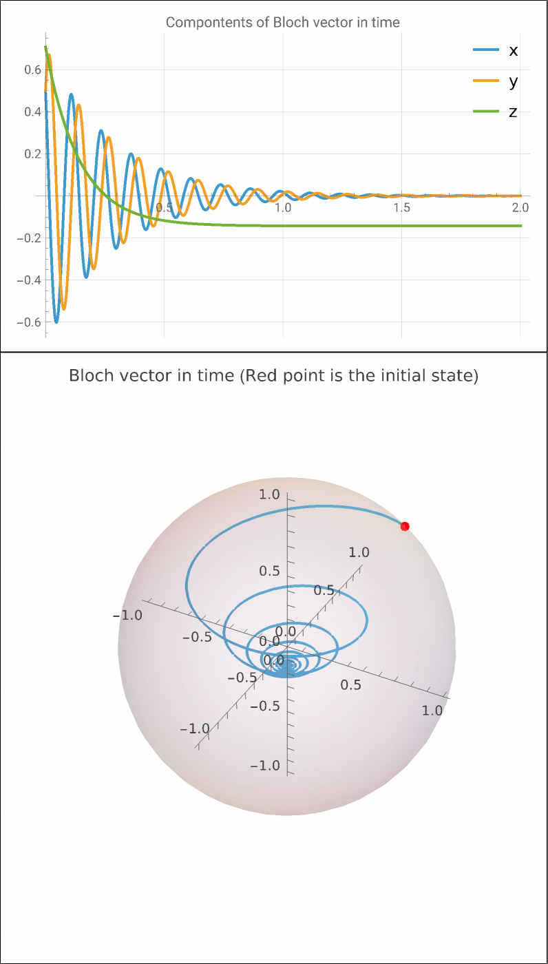
The first example is a qubit undergoes both relaxation to the ground state and excitation to the excited state due to interactions with a thermal environment, at finite temperature. The parameter Ω defines the qubit’s energy splitting, γ sets the characteristic system–bath coupling rate, and is the mean thermal photon number at the qubit transition frequency.
N
Set Ω, γ and N parameters in finite temperature amplitude damping mechanism:
In[]:=
Ω=50.;γ=1.;n=3.;γs=γ{n+1,n};
Setting up Hamiltonian, list of jump/Lindblad operator and their corresponding rates
In[]:=
h=Ω/2PauliMatrix[3];l=
γs
{{{0,0},{1,0}},{{0,1},{0,0}}};Schur decomposition of Lindbladian:
In[]:=
{qOp,tOp}=SchurDecomposition[N@ℒvec[h,l]]//Chop
Out[]=
{{{-0.707107,0.707107,0,0},{0,0,1.,0},{0,0,0,1.},{0.707107,0.707107,0,0}},{{-7.,1.,0,0},{0,0,0,0},{0,0,-3.5+50.,0},{0,0,0,-3.5-50.}}}
Double-check the decomposition:
In[]:=
N@ℒvec[h,l]==qOp.tOp.ConjugateTranspose[qOp]
Out[]=
True
Set the initial state vector and the corresponding vectorized density matrix:
In[]:=
v0={Cos[π/8],Exp[π/4]Sin[π/8]};r0=vectorize[KroneckerProduct[v0,Conjugate[v0]]];
Using Schur decomposition, find the time-evolved vectorized density matrix, using Schur decomposition:
In[]:=
r[t_]=qOp.MatrixExp[ttOp].ConjugateTranspose[qOp].r0//FullSimplify
Out[]=
0.428571+0.424982,(0.25+0.25),(0.25-0.25),0.571429-0.424982
-7.t
(-3.5+50.)t
(-3.5-50.)t
-7.t
Visualize the evolution:
Out[]=
Define a function for the two-time correlation function when Liouvillian is time-independent:
Just as a quick exploration, let’s do some analysis of eigensystems, very briefly.
Check eigenvalues are the same
Visualize the evolution:
For the two-time correlation function, in this case, we need to calculate the propagator first.
Define a function for the two-time correlation function when Liouvillian is time-dependent:
CITE THIS NOTEBOOK
CITE THIS NOTEBOOK
Liouville-space vectorization and Schur decomposition for Lindblad evolution
by Mohammad Bahrami
Wolfram Community, STAFF PICKS, August 13, 2025
https://community.wolfram.com/groups/-/m/t/3529901
by Mohammad Bahrami
Wolfram Community, STAFF PICKS, August 13, 2025
https://community.wolfram.com/groups/-/m/t/3529901