The goal is to show how the Lafler-Kinman string-lengths-based measure, which is built into the Wolfram Function Repository (WFR) item “IrregularPeriodogram”, can be made to more closely resemble an ordinary periodogram. This occurred to me after the function was published, so I intend to add an example along the lines we will show below.
Start by obtaining the resource function for irregular periodograms.
In[]:=
irregPG=ResourceFunction["IrregularPeriodogram"];
What properties can we query?
In[]:=
ResourceObject[irregPG]["Properties"]
Out[]=
{AllVersions,AutoUpdate,Categories,ContributorInformation,Definition,DefinitionNotebook,DefinitionNotebookObject,Description,Details,Documentation,DocumentationLink,DocumentationNotebook,DownloadedVersion,ExampleNotebook,ExampleNotebookObject,Function,FunctionLocation,Keywords,LatestUpdate,Name,Originator,Properties,RelatedSymbols,ReleaseDate,RepositoryLocation,ResourceLocations,ResourceObject,ResourceType,SeeAlso,ShortName,SourceMetadata,Symbol,SymbolName,TestReport,Usage,UUID,VerificationTests,Version,VersionInformation,VersionsAvailable,WolframLanguageVersionRequired}
Check the Usage:
In[]:=
ResourceObject[irregPG]["Usage"]
Out[]=
ResourceFunction["IrregularPeriodogram"][w,times,vals] computes the irregular periodogram at frequency for the given set of and .ResourceFunction["IrregularPeriodogram"][w,mat] computes the irregular periodogram for the set of time and value pairs in the two-column matrix .
w
times
vals
mat
Now we open the example notebook.
ResourceObject[irregPG]["ExampleNotebook"]
Out[]=
NotebookObject

I copied and pasted code from the first example to regenerate the data and some of the plots.
In[]:=
SeedRandom[11222333344444]data=Sort[Map[{#,Sin[#]+Cos[3*#]/2}&,RandomReal[{0,20},500]]];times=data[[All,1]];vals=data[[All,2]]-Mean[data[[All,2]]];ListPlot[Transpose[{times,vals}]]
Out[]=
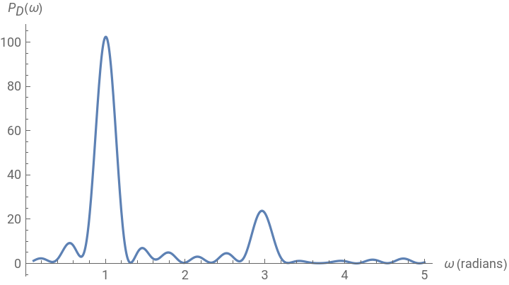
Plot[irregPG[w,times,vals],{w,.1,5},PlotPoints300,PlotRangeAll,AxesLabel{"ω (radians)","(ω)"}]
P
D
Out[]=
In[]:=
Plot[irregPG[p,times,vals,Method"LaflerKinman"],{p,1,8},PlotPoints300,PlotRangeAll,AxesLabel{"p","(p)"}]
P
LK
Out[]=
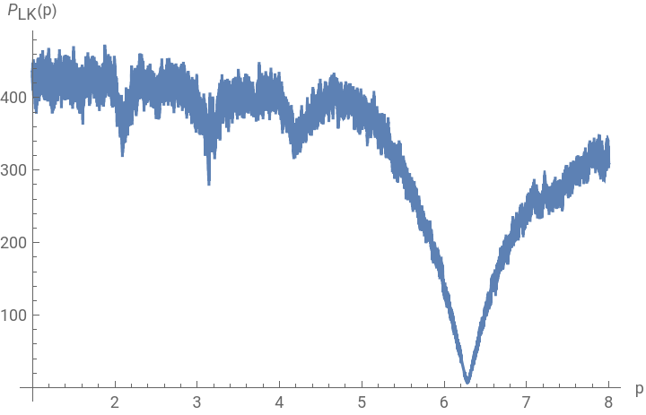
One will observe that this last is plotting putative period (that is, fold time span) against total string length. So instead of frequency on the horizontal axis we have time. And low rather than high values indicate points of interest. We go from time to frequency using the formula , and likewise go from small to large on the vertical axis by taking reciprocals.
f=2π/t
In[]:=
FrequencyAmplitude[{time_,len_}]:={2*Pi/time,1/len}
Generate a list of pairs.
{foldtime,magnitude}
In[]:=
pairs=Table[{p,irregPG[p,times,vals,Method"LaflerKinman"]},{p,1.,15,1/400}];
In[]:=
ListPlot[pairs]
Out[]=
Now do the transformation and re-plot.
In[]:=
ListPlot[Map[FrequencyAmplitude,pairs],PlotRangeAll]
Out[]=
We see that the main spike coincides with that of the Deeming periodogram. We also see a small bump in the Deeming periodogram near frequency 3. For the Lafler-Kinman version this corresponds to a fold time near 2.1:
In[]:=
NSolve[2.Pi/t3]
Out[]=
{{t2.0944}}
Home in to compute a lot of values in the vicinity of this folding time…
pairsNearby=Table[{p,irregPG[p,times,vals,Method"LaflerKinman"]},{p,1.85,2.3,1/10000}];ListPlot[Map[FrequencyAmplitude,pairsNearby],PlotRangeAll]
Out[]=
…and the bump has reappeared.