Introduction
Introduction
When I was planning an event for my university’s math club, one of my friends suggested that we host a generative art event, where guests can come and plot their own chaotic attractors; this was when I was introduced to generative art. I originally wanted to be a graphic designer, so you can imagine my excitement when I found out a way to combine my two interests: math and art. Non-linear dynamics is very interesting to visualize, however, for my pieces, I want to go beyond visualizing chaotic attractors. I did not know how to go about this until I looked at my current research projects in a more artistic perspective. These are my first attempts at generative art, and I wish to keep making more!
Kuramoto Model
Kuramoto Model
My current research is about the Kuramoto model in the context of computational neuroscience. The Kuramoto model is widely used to model synchrony in oscillator networks. The model is defined by+ϵsin-where (t)isthephaseofoscillator i at time t, is the natural frequency of the oscillator i, and is the coupling strength. This model can solved numerically, and we can observe that the system of oscillators will transition to synchrony over time. Here, we consider homogeneous natural frequency and a rotating frame. Thus the equations we will solve are
θ
i
ω
i
N
∑
j1
θ
j
θ
i
θ
i
ω
i
ϵ
Helper functions
Helper functions
First, let' s define some helper functions that solve the Kuramoto model . We choose uniformly random initial conditions chosen in the interval . Next, we solve the differential equation numerically with NDSolve. I override the KM function for the case with phase-lag and no phase-lag.
In[]:=
KM[ep_,tfinal_,timestep_, n_]:=Module[{phiInit,omega,trajs},Clear[phi]; Clear[t];SeedRandom[0];phiInit= RandomReal[{-Pi,Pi},n];trajs=NDSolve[{Table[{phi[i]'[t] ep/n Sum[Sin[phi[j][t]-phi[i][t]],{j,n}],phi[i][0]phiInit[[i]]},{i,n}]},Table[phi[i],{i,n}],{t,0,tfinal,timestep}]]
In[]:=
KM[ep_,tfinal_,timestep_, n_,phaselag_]:=Module[{phiInit,omega,trajs},Clear[phi]; Clear[t];SeedRandom[0]; phiInit= RandomReal[{-Pi,Pi},n];trajs=NDSolve[{Table[{phi[i]'[t] ep/n Sum[Sin[phi[j][t]-phi[i][t] - phaselag],{j,n}],phi[i][0]phiInit[[i]]},{i,n}]},Table[phi[i],{i,n}],{t,0,tfinal,timestep}]]
Next,wewillvisualizetheKuramotooscillators.Inthefirstfunction,weplotthephasesoftheoscillatorsasafunctionofindex.Additionally,inthesecondfunction,weplottheoscillatorsasapointsontheunitcircle,withthephasesusedastheargument.Thisideawillberelevanttohowtheartpiecesweremade.
In[]:=
visualizeKM[time_,trajs_]:=Module[{},Clear[phi]; Clear[t];ListPlot[Mod[Table[phi[jj][time]/.trajs,{jj,1,n}]//Flatten, 2*Pi], PlotRange{{1,n},{0,2*Pi}}]]
In[]:=
visualizeKMcirc[time_,trajs_]:=Module[{},Clear[phi]; Clear[t];Graphics[ComplexListPlot[Table[Exp[I*phi[jj][time]/.trajs],{jj,1,n}]//Flatten,Ticks None,PlotRange{{-1.25,1.25},{-1.25,1.25}},PlotStyle {RGBColor[0.79,0,0.5],PointSize[0.005]},LabelStyle{FontFamily"Academy Engraved LET",13,GrayLevel[0]}]]]
Investigating the model
Investigating the model
Consider a relatively small coupling strength, we can see that the oscillators synchronizes slowly .
In[]:=
ep=0.1;(*couplingstrength*)tfinal=100;(*simulating100seconds*)timestep=0.01;n=101;(*101oscillatorsconsidered*)(*Simulation*)trajs=KM[ep,tfinal,timestep,n];
In[]:=
Animate[visualizeKM[tt,trajs],{tt,0,tfinal},AnimationRunningFalse,SaveDefinitionsTrue]
Out[]=
In[]:=
Animate[visualizeKMcirc[tt,trajs],{tt,0,tfinal},AnimationRunningFalse,SaveDefinitionsTrue]
Out[]=
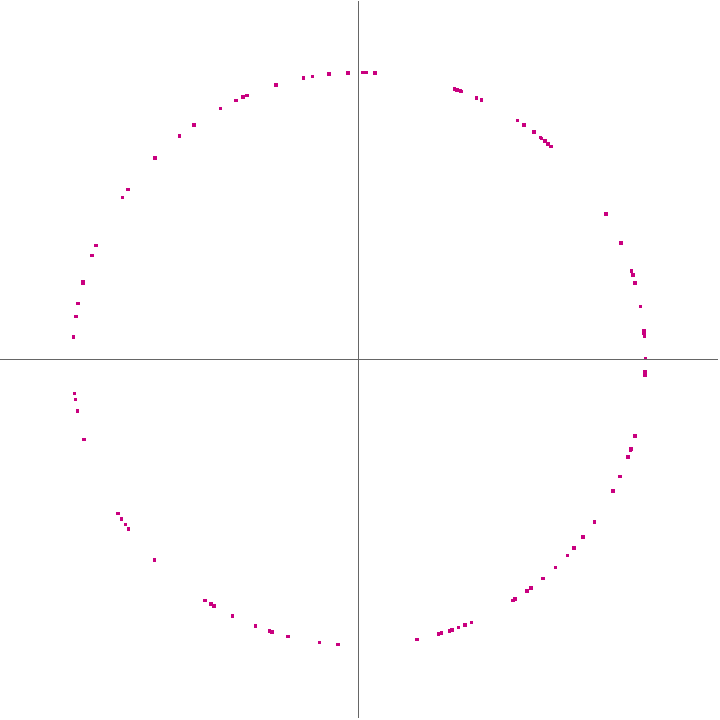
Choose a larger coupling strength, and the system synchronizes a lot quicker.
In[]:=
ep=1;(*couplingstrength*)(*Simulation*)trajs=KM[ep,tfinal,timestep,n];Animate[visualizeKMcirc[tt,trajs],{tt,0,tfinal},AnimationRunningFalse,SaveDefinitionsTrue]
Out[]=
Wecaninducemoreinterestingdynamicsbyintroducingphase-lagtothesystem,andthusthedefiningequationsbecomeWithappropriate,thesystemcanexhibitchimerastates,ortheexistenceofcoherentandincoherentclusters,andsomearguethatthisisachaoticattractor.
In[]:=
ep=0.1;phaselag=1.2;tfinal=500;trajs=KM[ep,tfinal,timestep,n,phaselag];Animate[visualizeKMcirc[tt,trajs],{tt,0,tfinal},AnimationRunningFalse,SaveDefinitionsTrue]
Code
Code
Parameters
Parameters
Generative Art Submissions
Generative Art Submissions
Submission 1
Submission 1
I decided to call this piece KM 39. I wanted to keep the color scheme minimal to focus on the intricate trajectories formed by these oscillators. Another look of the art piece:
Submission 2
Submission 2
I call this piece focus. The gradient is to emphasize that each dot tells us the angle of the the oscillator with respect to the horizontal axis.