ABSTRACT (original article): Mathematical Epidemiology (ME) shares with Chemical Reaction Network Theory (CRNT) the basic mathematical structure of its dynamical systems. Despite this central similarity, methods from CRNT have been seldom applied to solving problems in ME. We explore here the applicability of CRNT methods to find bifurcations at endemic equilibria of ME models. We adapt three CRNT methods to the features of ME. First, we prove that essentially all ME models admit Hopf bifurcations for certain monotone choices of the interaction functions. Second, we offer a parametrization of equilibria Jacobians of ME systems where few interactions are not in mass action form. Third, for a quite general class of models, we show that periodic oscillations in closed systems imply periodic oscillations when demography is added. Finally, we apply such results to two families of networks: a general SIR model with a nonlinear force of infection and treatment rate and a recent SIRnS model with a gradual increase in infectiousness. We give both necessary conditions and sufficient conditions for the occurrence of bifurcations at endemic equilibria of both families. CITATION (original article): Nicola Vassena, Florin Avram, Rim Adenane, Finding bifurcations in mathematical epidemiology via reaction network methods, arXiv:2310.19696. https://doi.org/10.48550/arXiv.2405.14576
Constants definition and numerical conditions
Constants definition and numerical conditions
Defining constants directly to speed up computation of numerical model.
ClearAll["Global‘*"]SetDirectory[NotebookDirectory[]];SetOptions[$FrontEndSession,NotebookAutoSave->True];NotebookSave[];Format[γr]:=Subscript[γ,r];Format[γs]:=Subscript[γ,s];Format[γi]:=Subscript[γ,i];Format[μr]:=Subscript[μ,r];Format[μs]:=Subscript[μ,s];Format[μi]:=Subscript[μ,i];sd=;R0= ;rd=Λ/μ-sd;b0=;cncut={λ->1+11ξ/10,a->(ξ-3)^2,b->ξ-4,γr->1,μr->1,μs->1/10,μi->2,β->1,γi->1,γs->1}(*Numericalconditionwithξkeptunknown*);csi={s->ξ,i->1}(*semi-numericalendemicpoint*);(*criticalvalueofξHwhenHopfbifurcationarise*)xiH=*4351-
λ(γr+μr)
γsμr+γrμs+μrμs
sdβ
a+γi+μi
(a+γi+μi)(γsμr+γrμs+μrμs)
λ(γr+μr)
1
620
584161
;We define the symbolic model using a stoichiometric matrix S and a vector of rates Vg, then we specialize the model in the case of non linear treatment function and linear incidence function:
In[]:=
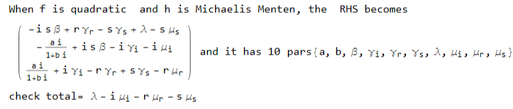
var={s,i,r};S={{1,-1,0,1,-1,-1,0,0},{0,1,-1,0,0,0,-1,0},{0,0,1,-1,1,0,0,-1}};(*Thestochiometricmatrix*)Vg={λ,f[s,i],h[i],γrr,γss,sμs,iμi,rμr};RHS=S.Vg;par=Complement[Variables[RHS],var];Print["The symbolic RHS ",RHS//MatrixForm," has ",par//Length," par given by ",par](*Thecaseofquadraticf(s,i)andMichaelisMentenh(i)*)cex={f[s,i]->βsi,h[i]->γii+ai/(1+bi)};RHSx=RHS//.cex;parx=Complement[Variables[RHSx],var];cpx=Thread[parx>0];RHSxn=RHSx//.cncutPrint["When f is quadratic and h is Michaelis Menten, the RHS becomes ",RHSx//MatrixForm," and it has ",parx//Length," pars",parx]Print["check total= ",Total[RHSx]//FullSimplify]
The symbolic RHS
has 8 par given by {,,λ,,,,f[s,i],h[i]}
r γ r γ s μ s |
-i μ i |
-r γ r γ s μ r |
γ
r
γ
s
μ
i
μ
r
μ
s
Out[]=
1+r--is+,-3i+is-,i-2r+s+
11s
10
11ξ
10
i
2
(-3+ξ)
1+i(-4+ξ)
i
2
(-3+ξ)
1+i(-4+ξ)
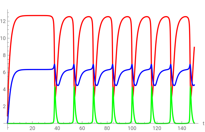
Time and parametric plots suggest the existence of periodic solutions at different values of ξ
Time and parametric plots suggest the existence of periodic solutions at different values of ξ
IIlustration of the time and phase plot when ξ=6 (when the eigenvalues
of the Jacobian at the unstable endemic point are (−2.33284, 0.116421 ± 1.23678 Im)) , suggest the existence of a stable limit cycle:
of the Jacobian at the unstable endemic point are (−2.33284, 0.116421 ± 1.23678 Im)) , suggest the existence of a stable limit cycle:
In[]:=
Xt=Map[#[t]&,var];ct=Thread[var->Xt];RHSt=RHSxn/.ct;ss=RHSt[[1]];ii=RHSt[[2]];rr=RHSt[[3]];T=150;c6={ξ->6};T1=50;X0={0.9,0.05,0.05};ode={s'[t]==ss,i'[t]==ii,r'[t]==rr,s[0]==X0[[1]],i[0]==X0[[2]],r[0]==X0[[3]]};odeN=ode/.c6;sol=NDSolve[odeN,var,{t,0,T}]plT=Plot[Evaluate@{s[t]/.sol,i[t]/.sol,r[t]/.sol},{t,0,T},PlotRangeFull,PlotStyle{Red,Green,Blue},AxesLabel{"t",""},PlotLegends{"s","i","r"}]pp=ParametricPlot[{s[t],i[t]}/.sol,{t,0,T1},AxesLabel{"s","i"},PlotStyle{Red},Epilog->{{PointSize[Large],Point[{X0[[1]],X0[[2]]}]},Text["(,)",Offset[{10,8},{X0[[1]],X0[[2]]}]]},AxesOrigin{0,0}];Show[pp,PlotRange->All];Export["plT6.pdf",plT]
s
0
i
0
Out[]=
sInterpolatingFunction,iInterpolatingFunction,rInterpolatingFunction


Out[]=


Out[]=
plT6.pdf
We produce now parametric plots when ξ=6 suggesting convergence to a limit cycle around the endemic point, both when starting from inside and outside the cycle. Note the apparent intersection between the paths is due to the fact that we are projecting three dimensional paths in two dimensions.
In[]:=
(*Nowbystratingfrominsidethecycle*)X02={7,2,1.5}(*Differentinitialvalues*);ode={s'[t]==ss,i'[t]==ii,r'[t]==rr,s[0]==X02[[1]],i[0]==X02[[2]],r[0]==X02[[3]]};T=300;odeN=ode/.c6;sol=NDSolve[odeN,var,{t,0,T}];pp1=ParametricPlot[{s[t],i[t]}/.sol,{t,0,T},AxesLabel{"s","i"},PlotRangeFull,PlotStyle{Dashed,Blue}];(*Nowbystratingagainfromoutsidethecycle*)X03={10,2,1.5}(*Differentinitialvalues*);ode={s'[t]==ss,i'[t]==ii,r'[t]==rr,s[0]==X03[[1]],i[0]==X03[[2]],r[0]==X03[[3]]};T=300;odeN=ode/.c6;sol=NDSolve[odeN,var,{t,0,T}];pp2=ParametricPlot[{s[t],i[t]}/.sol,{t,0,T},AxesLabel{"s","i"},PlotRangeFull,PlotStyle{Dashed,Magenta}];pyn=Plot[(1),{t,0,12},PlotStyle{Dashed,Green}](*plotofthevalueofendemici*);Print["The unstable endemic point has the following coordinates "]fp={ξ,1}//.c6//NppF=Show[{pp,pp1,pp2,Graphics[{Green,Dashed,Line[{{fp[[1]],0},{fp[[1]],4.5}}]}],pyn},Epilog{Text["(,)",Offset[{10,8},{X0[[1]],X0[[2]]}]],{PointSize[Large],Point[{X0[[1]],X0[[2]]}]},{Text["(,)",Offset[{10,-8},{(fp[[1]]),(fp[[2]])}]],{PointSize[Large],Style[Point[{(fp[[1]]),(fp[[2]])}],Cyan]}},{PointSize[Large],Point[{X02[[1]],X02[[2]]}]},Text["(',')",Offset[{10,-8},{X02[[1]],X02[[2]]}]],{PointSize[Large],Point[{X03[[1]],X03[[2]]}]},Text["('','')",Offset[{10,-8},{X03[[1]],X03[[2]]}]]},PlotRange->All]Export["ppF.pdf",ppF]
s
0
i
0
s
*
i
*
s
0
i
0
s
0
i
0
IIlustration of the time plot when ξ=ξH ( the eigenvalues of the Jacobian at the endemic point are (−2.31501, ±1.29094 Im)) suggest the existence of a unique limit cycle :
In the following, we chose different starting points, and we illustrate the time plots of s from different initial points. This suggests again the existence of a unique limit cycle:
Analysis of the saddle node bifurcation dis=0:
Analysis of the saddle node bifurcation dis=0:
In this cell we give an alternative solution to the zero eigenvalue bifurcation point, using also the script RUR in our package Epid, which reduces the fixed point system to a scalar polynomial. This allows also a quick computation of a Bogdanov-Takens point.
CITE THIS NOTEBOOK
CITE THIS NOTEBOOK
Finding bifurcations in mathematical epidemiology via reaction network methods
by N. Vassena, F. Avram, and R. Adenane
Wolfram Community, STAFF PICKS, June 5, 2024
https://community.wolfram.com/groups/-/m/t/3188310
by N. Vassena, F. Avram, and R. Adenane
Wolfram Community, STAFF PICKS, June 5, 2024
https://community.wolfram.com/groups/-/m/t/3188310