Two famous eruptions, two scales of the same physics, side by side. LEFT: Eyjafjallajökull 2010 – the ash that closed European airspace – modelled on the REAL April-2010 reanalysis winds, the fine-ash veil (cyan) fanning out of Iceland on the genuine jet, with the real wind drawn beneath as a flow texture (line-integral convolution) coloured by speed (§10). RIGHT: two centuries on and a thousand times larger – the Tambora 1815 sulfate veil wrapping a rotating globe over a year (§11). The same size-resolved particle model runs from a single live advisory to a planet-dimming catastrophe.
When a volcano erupts, the world's nine Volcanic Ash Advisory Centres (VAACs) issue short, free text bulletins – Volcanic Ash Advisories – giving the observed ash-cloud polygon, its flight-level band, and a forecast of where it will be in 6, 12 and 18 hours. This notebook turns those bulletins into a quantitative forecast: a single generic parser reads the bulletins from three different centres (Tokyo, London, Toulouse), and we advect the ash polygon with free ERA5 reanalysis winds at flight levels from Open-Meteo. For the live Sheveluch eruption the wind-advected polygon lands about 8 km from the VAAC's own +6 h forecast, against 112 km for a no-wind (persistence) guess. We then go beyond the outline with a Lagrangian particle model: thousands of ash grains carried by the wind at their own altitude and settling at their size-dependent fall speed, so coarse ash drops out at the vent while fine ash is driven hundreds of km downwind – and the same source at different flight levels fans out, the vertical wind shear that makes a single map of an ash cloud dangerous for aviation.
1. Why volcanic ash matters to aviation
1. Why volcanic ash matters to aviation
Volcanic ash is pulverised rock and glass, melting around 1100 °C – well below a jet engine's combustor temperature. Ingested ash melts, then re-solidifies on the cooler turbine blades, choking airflow and stalling the engine; it also sandblasts windscreens and clogs the pitot tubes that measure airspeed. In 1982 British Airways Flight 9 flew into a Galunggung ash cloud at night and lost all four engines (they restarted only after gliding out below the cloud); in 2010 Eyjafjallajökull shut European airspace for six days.
Because the hazard is invisible to radar and often to the naked eye, ash is tracked from geostationary satellites using the "reverse absorption" or split-window technique: silicate ash and water/ice cloud have opposite brightness-temperature differences between two thermal-infrared channels (around 11 and 12 μm), which lets an algorithm flag ash. Nine Volcanic Ash Advisory Centres (Tokyo, London, Toulouse, Anchorage, Washington, Montreal, Darwin, Wellington, Buenos Aires) divide the globe between them. When ash is detected the responsible centre issues a Volcanic Ash Advisory (VAA) – a terse text bulletin – and reissues it, usually every 6 hours, until the sky is clear.
2. The Volcanic Ash Advisory text format
2. The Volcanic Ash Advisory text format
A VAA is a fixed-field telex-style message. Here is the live Tokyo VAAC bulletin for Sheveluch (Kamchatka) that this notebook is built around – note the observed cloud line OBS VA CLD with its flight-level band SFC/FL220, the polygon vertices in degrees-and-minutes, the drift MOV NW 10KT, and the +6/+12/+18 h forecast polygons:
FVFE01 RJTD 021800VA ADVISORYDTG: 20260602/1800ZVAAC: TOKYOVOLCANO: SHEVELUCH 300270PSN: N5639 E16122AREA: RUSSIASOURCE ELEV: 3283M AMSLADVISORY NR: 2026/159INFO SOURCE: HIMAWARI-9ERUPTION DETAILS: VA CONTINUOUSLY OBS IN SATELLITE IMAGERYOBS VA DTG: 02/1720ZOBS VA CLD: SFC/FL220 N6325 E15214 - N6216 E15053 - N5728 E15256 - N5653 E15234 - N6214 E15005 - N6330 E15149 MOV NW 10KTFCST VA CLD +6 HR: 02/2320Z SFC/FL230 N6413 E15212 - N6256 E15019 - N6056 E15206 - N5836 E15116 - N6223 E14723FCST VA CLD +12 HR: 03/0520Z SFC/FL220 N6507 E15217 - N6339 E15007 - N6237 E15229 - N6049 E14921 - N6230 E14333FCST VA CLD +18 HR: NO VA EXPRMK: SOME PART OF VA OBSCURED BY MET CLOUD.NXT ADVISORY: 20260603/0000Z=
Every centre issues this same grammar, but the surface form differs: Tokyo strips to one line, London puts each field on its own line, Toulouse emits clean FIELD: value lines. One parser handles all three.
3. Parsing the advisory
3. Parsing the advisory
ParseVAAdvisory locates each field label wherever it appears and returns a structured association. First the one-time setup that loads the helper package and the embedded data:
(*one-timesetup:loadthehelperpackageandtheembeddeddata*)SetDirectory[NotebookDirectory[]];Get["plume_dispersion_helpers.wl"];sheveluchText=;bardarbungaText=;sakurajimaText=;etnaText=;pShev=ParseVAAdvisory[sheveluchText];pBard=ParseVAAdvisory[bardarbungaText];pSaku=ParseVAAdvisory[sakurajimaText];pEtna=ParseVAAdvisory[etnaText];(*Open-MeteoERA5windsnapshot,embeddedinline*)windData=Uncompress;field=WindFieldFromData[windData];obsPoly=pShev["obs"]["layers"][[1]]["polygon"];steer=SteeringLevel[field,pShev];(*Lagrangianparticlecloud:grains,18h,snapshotsevery90min*)snaps=EvolveParticles[field,pShev,4200,18,15,45];shevRange=Module[{ps=Join@@Table[Transpose[{s["state"]["lat"],s["state"]["lon"]}],{s,snaps}]},{{Min[ps[[All,1]]]-0.5,Max[ps[[All,1]]]+0.5},{Min[ps[[All,2]]]-0.5,Max[ps[[All,2]]]+0.5}}];ptcl=Last[snaps]["state"];(*realzonal-mean50hPawindprofile(ERA5,amodernproxyfor1815)*)stratProfile={{-80,17.5},{-70,28.7},{-60,34.},{-50,31.1},{-40,21.4},{-30,10.1},{-20,1.4},{-10,-13.5},{0,-18.4},{10,-19.6},{20,-11.4},{30,-6.2},{40,-1.9},{50,-2.3},{60,-3.1},{70,-0.1},{80,1.5}};SetStratProfile[stratProfile];
loaded – wind field levels (hPa): {150.,200.,250.,300.,400.,500.,600.,700.,850.}
The coordinate parser turns degrees-and-minutes into signed decimal degrees:
ParseCoord["N5639","E16122"]
{56.65,161.367}
The parsed header and the observed ash layer (flight-level band, polygon and reported drift):
Dataset@KeyTake[pShev,{"volcano","vaac","area","position","obsDTG"}]
pShev["obs"]["layers"][[1]]
flLow0,flHigh220,polygon{{63.4167,152.233},{62.2667,150.883},{57.4667,152.933},{56.8833,152.567},{62.2333,150.083},{63.5,151.817}},movDirNW,movKt10,movBearing315
Plotted on a map, the observed cloud (filled) and the VAAC's own +6/+12/+18 h forecast polygons (outlines):
AdvisoryMap[pShev]
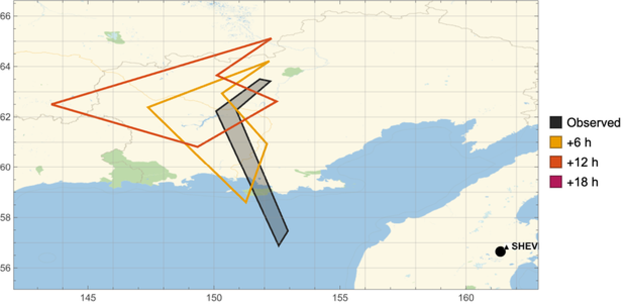
These angular, sometimes bow-tie-shaped outlines are the VAAC polygons exactly as issued: the centre lists a handful of vertices in advisory order, so the boundary can look jagged or self-crossing. The polygon is only the cloud's outline – it says nothing about what is inside. §7 fills it in with physics.
4. Winds at flight levels
4. Winds at flight levels
A flight level is an altitude in hundreds of feet at the standard-pressure datum. We map it to a pressure surface through the ICAO Standard Atmosphere
p(h)=1013.25hPa
5.25588
(1-2.25577×h)
-5
10
Why pressure? Meteorologists use pressure, not metres, as the vertical coordinate, because winds are archived on pressure surfaces. We therefore convert a flight level to an altitude, then to a pressure, and snap to the nearest level the free, key-less Open-Meteo ERA5/IFS pressure-level API serves. FL220 works out at about 430 hPa, which snaps to the 400 hPa level:
{FlightLevelToPressure[220],SnapLevel[FlightLevelToPressure[220]]}
{427.914,400}
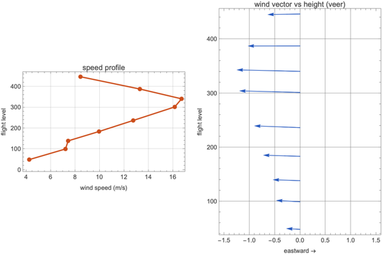
Winds change dramatically with height – this is why the flight level of an ash cloud matters so much. Near the surface friction makes them light and variable; at cruise altitude they organise into the jet stream, where speeds routinely exceed 50 m/s. The wind at a given point, flight level and time (eastward u, northward v, in m/s) is read straight from the interpolated reanalysis field, which the package builds as a 3-D interpolation over time, latitude and longitude for each pressure level:
WindAt[field,60.,156.,300.,pShev["obsDTG"]]
{-7.8033,10.3627}
Across the column the wind both strengthens and veers with height – the speed profile and the wind vector at each flight level:
WindProfilePlot[field,Sequence@@pShev["position"],pShev["obsDTG"]]
5. Advecting the plume
5. Advecting the plume
"Advection" just means transport by the wind. We treat it Lagrangian-ly – following parcels of air rather than watching fixed points – so we carry each polygon vertex along with the local wind. To convert a wind in m/s into a change of latitude/longitude we divide by the length of a degree (about 111 km), with a cos(latitude) correction for longitude because meridians converge toward the poles. We use a midpoint (RK2) step: sample the wind, take a half step, re-sample, then take the full step from there – more accurate than a naive Euler step when the wind varies along the path. Per step:
Δϕ=,Δλ=cosϕ
vΔt
R
ϕ
uΔt
R
ϕ
A cloud labelled SFC/FL220 fills 6 km of atmosphere, and every level in that column moves differently – so which one steers the cloud the satellite actually sees? We let the data decide: of all available pressure levels in that band we pick the one whose reanalysis wind best matches the VAAC's reported drift vector (MOV NW 10KT), the "steering level", and advect there. For Sheveluch that comes out at the lowest level the free pressure-level API serves in this band, ~850 hPa – consistent with the gentle 10-knot drift the forecaster reported:
{steer,SnapLevel[steer],WindAt[field,Sequence@@pShev["position"],steer,pShev["obsDTG"]]}
{850.,850,{-3.53067,2.38705}}
CentroidLatLon@AdvectPolygon[field,obsPoly,steer,pShev["obsDTG"],6]
{61.8383,150.793}
6. Skill: does the wind beat persistence?
6. Skill: does the wind beat persistence?
We score our wind-advected polygon against the VAAC forecaster's own polygon at each lead time – centroid great-circle error, the same error for a no-wind persistence guess, and the polygon overlap (intersection-over-union):
On the map, our wind-advected polygons (dashed) track the VAAC's forecast polygons (solid):
7. Beyond the outline: ash as moving particles
7. Beyond the outline: ash as moving particles
The polygon is just a boundary. What is physically there is a cloud of ash grains spanning a huge size range – from sub-10 μm dust to millimetre lapilli – and size controls everything. A grain falls at its terminal velocity, where gravity balances aerodynamic drag. For the smallest grains the air flows smoothly around them and drag is linear in speed (Stokes' law, fall speed ∝ diameter squared); larger grains stir turbulent wakes and fall more slowly than Stokes would predict. We solve the full drag balance (Clift–Gauvin) at each grain's altitude – thinner air aloft means less drag – and the fall speed grows steeply with diameter, from millimetres per second to metres per second:
So we seed an eruption column at the vent (a few thousand grains, log-normal sizes) and step each one forward (a simple explicit step every 15 min) with the wind at its CURRENT altitude, gravitational settling, and a turbulent random walk. Large grains plunge out within minutes; fine ash rides the wind for hours. Here is the whole 18-hour evolution as a glowing animation over the gray relief of Kamchatka – every grain sized and coloured by diameter – coarse ash settles out near the vent while the cyan fine-ash veil streams downwind, the densest part of the cloud glowing white-hot. Beneath it, the real ERA5 steering-level wind is drawn as a line-integral-convolution texture coloured by true speed – note how gentle the flow is (only a few m/s) yet enough to carry the fine ash hundreds of km:
The Lagrangian ash cloud over 18 h, in the same glowing style as the hero: coarse grains settle out near Sheveluch while the fine-ash veil (cyan) rides the ERA5 winds – shown beneath as an LIC flow texture coloured by the real (gentle) wind speed – hundreds of km downwind.
Counting how many particles sit in each map cell gives the airborne density – a physical concentration field, not just an outline:
The size sorting is stark: distance carried versus grain diameter falls off by two orders of magnitude. Coarse ash deposits within ~10 km of the vent; the finest is still aloft 300–500 km downwind:
And the cloud changes character with time: the coarse and medium fractions settle out within a few hours, leaving an increasingly fine-grained plume – exactly the long-lived fine ash that closes airspace:
This is the same size-resolved particle model that drives the hero animation at the top of this notebook and the Eyjafjallajökull case in §10 – here on a single live advisory.
8. Vertical wind shear – the hazard a single map hides
8. Vertical wind shear – the hazard a single map hides
Because the wind veers with height, the same source advected at different flight levels goes to different places. A controller looking at one altitude sees only part of the threat:
The London VAAC encodes this directly: its bulletins can carry several flight-level bands, each with its own polygon and drift. The Bárðarbunga exercise message below has three (SFC/FL200, FL200/350, FL350/550):
London VAAC exercise / product-test message – used here only because it carries a realistic multi-layer polygon set.
9. Three volcanoes, three centres, one parser
9. Three volcanoes, three centres, one parser
The brief named Sakurajima, the Reykjanes peninsula and Etna. In early June 2026 each is in a different state, which is itself instructive. Sakurajima (Tokyo VAAC) is in its routine small-puff mode – dozens of short ash emissions a month, each too small or short-lived to track as a polygon. Iceland (London VAAC) is quiet, so the only traffic is the centre's periodic exercise / product-test messages. Etna (Toulouse VAAC) is on aviation colour code GREEN with no ash. The same parser reads all three, and where there is no trackable cloud it still extracts the reported eruption-level wind and the status – so even a "quiet" panel tells you something:
10. A famous case: Eyjafjallajökull, 2010
10. A famous case: Eyjafjallajökull, 2010
The eruption everyone remembers is Eyjafjallajökull (Iceland, April–May 2010). It was not large by volcanic standards, but a fine, glassy ash plume rode the jet stream straight into the busiest airspace on Earth. Over six days ~100,000 flights were cancelled and ~10 million passengers stranded – the largest air-traffic shutdown since 1945. Open-Meteo's archive has no flight-level winds this far back, but the NCEP/NCAR Reanalysis does (free, no key, hourly back to 1948), so this time we drive the particle model with the REAL April-2010 winds – downloaded straight from the NOAA THREDDS server. And because the volcano did not puff once but erupted for weeks, we inject fresh ash at the vent continuously, so the model builds a sustained, fanning plume rather than a single dispersing cloud:
A SUSTAINED eruption driven by the REAL April-2010 reanalysis winds: fresh ash injected at the vent streams out on the genuine jet (here ~40 m/s at the vent, eastward), the fine-ash veil (cyan) fanning across the North Atlantic toward Britain and Scandinavia as the winds veer day to day – the real flow drawn beneath as an LIC texture coloured by wind speed, with direction arrows. Not an idealization: this is what the atmosphere actually did.
Now a genuine skill check. Take everywhere the ash was airborne over the whole episode – its swept footprint – and compare it with the countries that actually closed their airspace 15–21 April 2010:
Modelled swept ash (cyan) vs the countries that closed their airspace 15–21 April 2010 (amber, documented). Driven by the real winds, the modelled veil reaches 8 of those 18 countries – Britain, Ireland, the North Sea coasts and Scandinavia. Much of the airborne mass rides the jet out over the open Atlantic (so a strict area overlap is modest), and our single plume-top column cannot capture the full multi-level, multi-day spread that grounded central Europe too – but with genuine reanalysis winds the model puts the ash over the right places, for the right reason.
11. Tambora 1815: how the dust went around the world
11. Tambora 1815: how the dust went around the world
Step back two centuries. In April 1815 Mount Tambora (Indonesia) produced the largest eruption in recorded history – VEI 7, roughly a hundred times Eyjafjallajökull. The danger then was not jet engines but the climate. Tambora injected ~60 million tonnes of sulfur dioxide into the STRATOSPHERE, where it converted to a fine sulfate-aerosol haze. Unlike tropospheric ash, stratospheric aerosol does not rain out in days; it lingers for one to three years, scatters sunlight back to space, and spreads across the entire planet. The result was 1816, the "Year Without a Summer": snow in New England in June, failed harvests across Europe, food riots and famine – and, indirectly, red sunsets in Turner's paintings and a wet Swiss summer that kept Mary Shelley indoors writing Frankenstein.
1815 is far beyond any wind dataset, so we cannot use the winds of the time. But the relevant transport is stratospheric, and the stratosphere's circulation is dominated by a few robust, slowly-varying features – so we drive the tracers with a REAL zonal-mean wind profile measured at 50 hPa (~20 km) from today's reanalysis, as a modern proxy. Two processes do the work. A strong, latitude-dependent ZONAL wind – equatorial easterlies (here in their easterly phase; the real Quasi-Biennial Oscillation reverses every ~28 months) flanked by mid-latitude jets, the winter polar-vortex jet reaching ~35 m/s – wraps aerosol around the globe in a couple of weeks. A slow POLEWARD drift (the Brewer–Dobson circulation) plus mixing then fills both hemispheres over months. The real zonal-mean wind we use, by latitude (note the easterly tropics and the strong southern jet):
Releasing 12,000 tracers at Tambora and integrating for a year on a slowly rotating globe, the glowing veil first streaks around the tropics, then bleeds poleward into both hemispheres until it covers the planet:
Stratospheric tracer model on a rotating globe, driven by a real zonal-mean 50 hPa wind profile (a modern proxy; 1815's own winds are unknown). The Tambora veil wraps the tropics in ~2 weeks, then spreads to both hemispheres over months.
Quantitatively, the tropical belt is encircled within about two weeks and the whole globe within a few months – the timescale on which Tambora's veil dimmed the sun worldwide and chilled the summer of 1816:
12. Caveats
12. Caveats
Three models live here, in increasing order of abstraction: a polygon advection (§5–6), a Lagrangian particle model (§7–10), and the schematic global tracer model (§11). All are simpler than the operational dispersion models (NAME, HYSPLIT, FALL3D). The particle model uses spherical-grain drag, a prescribed log-normal size distribution and a constant eddy diffusivity; it ignores aggregation, the ash/SO₂ distinction, plume-rise dynamics and wet deposition. The Tambora model uses a real zonal-mean 50 hPa wind profile but from today, not 1815 (none exists for 1815), keeps a parameterized poleward drift, and is meant to convey the PROCESS and its timescales, not a forecast. The aim throughout is to show, reproducibly and mostly from free data, how far wind plus elementary physics already take you.
13. References & data
13. References & data
VAA bulletins: Tokyo VAAC (JMA), London VAAC (Met Office), Toulouse VAAC (Météo-France). Winds: Open-Meteo ERA5/IFS pressure-level API (CC BY 4.0). ICAO Doc 9766 (Handbook on the IAVW). Settling: Clift & Gauvin drag. Eyjafjallajökull 2010 winds: NCEP/NCAR Reanalysis-1 (Kalnay et al. 1996, NOAA PSL), pressure-level, no key. Eyjafjallajökull 2010 impact figures: Eurocontrol / IATA. Tambora & the Year Without a Summer: Stommel & Stommel (1983), Oppenheimer (2003); its stratospheric transport is driven by a real zonal-mean 50 hPa wind profile from today's reanalysis used as a schematic proxy. The Bardarbunga advisory shown is a London VAAC exercise message.
14. Reproducibility
14. Reproducibility
The whole pipeline is pure Wolfram Language:
wolframscript -file wolfram/fetch_all.wls (* refresh advisory + wind snapshots *)
wolframscript -file wolfram/run_all.wls (* render docs/images/*.png + hero *)
wolframscript -file community/build_notebook.wls (* assemble this notebook *)
wolframscript -file wolfram/run_all.wls (* render docs/images/*.png + hero *)
wolframscript -file community/build_notebook.wls (* assemble this notebook *)
This notebook is self-contained: the advisory texts and the wind snapshot are embedded above, so every cell re-runs without any external file (map backgrounds excepted, which fetch tiles).
CITE THIS NOTEBOOK
CITE THIS NOTEBOOK
VAAC ash-cloud bulletin parsing & ERA5 flight-level advection for volcanic plume dispersion
by Marco Thiel
Wolfram Community, STAFF PICKS, June 12, 2026
https://community.wolfram.com/groups/-/m/t/3732387
by Marco Thiel
Wolfram Community, STAFF PICKS, June 12, 2026
https://community.wolfram.com/groups/-/m/t/3732387