ORIGINAL BOOK: Seiichi Nomura (2022), Complex Variables for Engineers with Mathematica, Springer Cham.
ISBN: 978-3-031-13067-0. DOI: https://doi.org/10.1007/978-3-031-13067-0
ISBN: 978-3-031-13067-0. DOI: https://doi.org/10.1007/978-3-031-13067-0
I have been using Mathematica since it became available on the NeXT computer. Mathematica is invaluable in my field, micromechanics, where one frequently needs to manipulate complex tensor algebra. I have also utilized Mathematica as a teaching tool and have found it exceptionally useful in handling complex variables, with specific applications to engineering problems such as heat conduction, elasticity, and fluid mechanics.
In this notebook, I’ve included examples from the three areas mentioned above to demonstrate how Mathematica can simplify otherwise tedious calculations. In heat conduction, I addressed the temperature distribution in a two-phase medium subjected to uniform heat flux. For solid mechanics, I examined the stress field in a plate with a hole under far-field tension. In fluid mechanics, I’ve provided a sample Mathematica code to visualize the streamlines of an incompressible fluid.
In this notebook, I’ve included examples from the three areas mentioned above to demonstrate how Mathematica can simplify otherwise tedious calculations. In heat conduction, I addressed the temperature distribution in a two-phase medium subjected to uniform heat flux. For solid mechanics, I examined the stress field in a plate with a hole under far-field tension. In fluid mechanics, I’ve provided a sample Mathematica code to visualize the streamlines of an incompressible fluid.
A complex function can be visualized by looking at its absolute value using Plot3D[]. The following shows the behavior of which shows a singularity at .
f(z)exp-
1
2
z
z0
In[]:=
z=x+Iy;Plot3D[Abs[Exp[-1/z^2]],{x,-1,1},{y,-1,1}]
Out[]=

Plotting on the complex plane shows that the absolute value of goes beyond 1.
sinz
sinz
In[]:=
Plot3D[Abs[Sin[z]],{x,-3,3},{y,-5,5}]
Out[]=

Heat Conduction
Heat Conduction
In steady-state heat conduction, the temperature, , is governed by the Laplace equation, along with the boundary condition. As the real part of an analytic function, , automatically satisfies the Laplace equation, one can expand by the Taylor series in the region where there is no singularities or by the Laurent series in the region where there are singularities such as a hole and take the real part of to derive a function satisfying the Laplace equation. The unknown coefficients of the expansion can chosen so that the boundary condition can be satisfied.
As an example, consider steady-state heat conduction in a half-plane outside a cylinder with a radius of 1/2 as shown below. The boundary condition is that along and along the wall of the cylinder. It is assumed that where and are unknown complex coefficients.
T
ΔT0
f(z)
f(z)
f(z)
As an example, consider steady-state heat conduction in a half-plane outside a cylinder with a radius of 1/2 as shown below. The boundary condition is that
TC
◦
100
x0
TC
◦
50
f(z)+/z
c
0
c
1
c
0
c
1
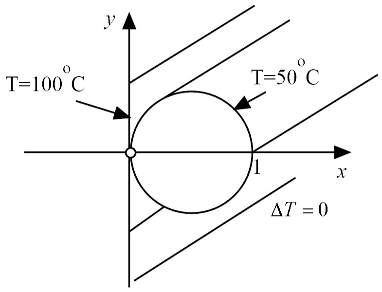

The following Mathematica code solves for and .
c
0
c
1
In[]:=
f=(a+bI)+(c+dI)/(x+Iy)t1=ComplexExpand[Re[f]]t1/.x0sol1={a100,d0}t1/.x^2+y^2xsol2={d0,c-50}temp=t1/.sol1/.sol2Plot3D[temp,{x,0,2},{y,-2,2}]
Out[]=
a+b+
c+d
x+y
Out[]=
a++++
cx
2
x
2
y
dy
2
x
2
y
Out[]=
a+
d
y
Out[]=
{a100,d0}
Out[]=
a+c+
dy
x
Out[]=
{d0,c-50}
Out[]=
100-+
50x
2
x
2
y
Out[]=

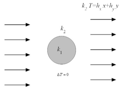
As a second example, heat conduction in a two-phase material is considered. A cylinder with thermal conductivity, . is placed in an infinitely extended medium with thermal conductivity, , subject to constant heat flux at infinity as shown in the figure below.The boundary condition is such that as , the heat flux is constant, i.e., asx,y∞.The temperature distribution, , inside the cylinder is expressed by the Taylor series while the temperature distribution, , in the surrounding medium can be expressed by the Laurent series asℜ+z+,ℜ++z+.The temperature distributions, and , must satisfy the continuity conditions of the temperature and heat flux at (radius) aswhere≡+The following Mathematica code can solve for the unknowns as0+(-i)-(-)(+i)(+)-i(z)+z,(z)(-)(+i)(+)+-iz+(x+y),1-(-)+x+y.
k
1
k
2
x,y∞
k
2
∂T
∂x
h
x
k
2
∂T
∂y
h
y
T
1
T
2
T
1
c
0
c
1
c
2
2
z
T
2
d
0
z
d
1
d
2
d
3
2
z
T
1
T
2
ra
T
1
T
2
k
1
∂
T
1
∂n
k
2
∂
T
2
∂n
∂T
∂n
x
a
∂T
∂x
y
a
∂T
∂y
c
0
c
2
d
1
d
3
c
1
2
k
1
k
2
h
x
h
y
d
0
2
a
k
1
k
2
h
x
h
y
k
2
k
1
k
2
d
2
h
x
h
y
k
2
f
1
2(-i)
h
x
h
y
k
1
k
2
f
2
2
a
k
2
k
1
h
x
h
y
k
2
k
1
k
2
1
z
h
x
h
y
k
2
T
1
2
k
1
k
2
h
x
h
y
T
2
2
a
k
1
k
2
(+)
k
1
k
2
1
2
x
2
y
h
x
h
y
k
2
Solid Mechanics
Solid Mechanics
As an example, consider an infinite plate with a hole at the center subject to uniform stresses at the far filed shown below.
The function, AiryStress[f,g], returns the stress components for two analytic functions, f and g. The function AiryDisplacement[f,g,kappa, mu] returns the displacements for two analytic functions, f and g, along with two material parameters, kappa and mu.
Fluid Mechanics
Fluid Mechanics
Here is a flow around a cylinder under a uniform flow.
CITE THIS NOTEBOOK
CITE THIS NOTEBOOK
Complex Variables for Engineers with Mathematica
by Seiichi Nomura
Wolfram Community, STAFF PICKS, October 27, 2023
https://community.wolfram.com/groups/-/m/t/3056789
by Seiichi Nomura
Wolfram Community, STAFF PICKS, October 27, 2023
https://community.wolfram.com/groups/-/m/t/3056789