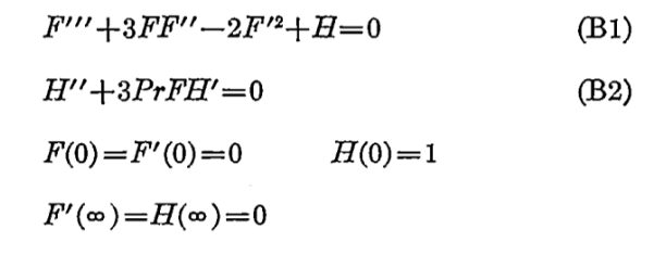
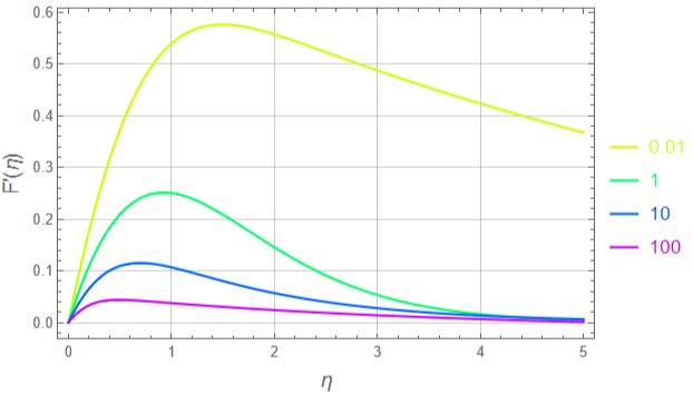
We compute the velocity and temperature profiles for free convection past an isothermal vertical plate. This problem was solved originally by Ostrach (see Ref. 1). Results are obtained after solving two coupled nonlinear differential equations. First, the shooting method is used to obtain the boundary conditions, required to solve the coupled ODEs, which match the conditions in the outer fluid. Then, we plot the velocity and temperature profiles versus a similarity variable for different values of the Prandtl numbers (Pr = 0.01, 1, 10 and 100). Derivation of the governing equations can be found in Deen' s book.
The governing equations are taken from Ref. 1 (Appendix B) :
In[]:=
Off[General::"spell1"]Off[NDSolve::"ndsz"]Off[InterpolatingFunction::"dmval"]Off[FindRoot::"lstol"]Off[FindRoot::"cvmit"]
Case 1: Prandtl number Pr = 1
In[]:=
Pr=1;
In[]:=
sol[ξ_,ψ_]:=NDSolve[{D[F[η],{η,3}]+3F[η]D[F[η],{η,2}]-2D[F[η],{η,1}]^2+θ[η]0,D[θ[η],{η,2}]+3PrF[η]D[θ[η],{η,1}]0,F[0]0,F'[0]0,θ[0]1,F''[0]ξ,θ'[0]ψ},{F[η],θ[η]},{η,0,10}]
In[]:=
θEnd[ξ_?NumericQ,ψ_?NumericQ]:=θ[η]/.sol[ξ,ψ]/.η10
In[]:=
DFEnd[ξ_?NumericQ,ψ_?NumericQ]:=(D[F[η]/.sol[ξ,ψ],{η,1}]^2/.η10)+(D[F[η]/.sol[ξ,ψ],{η,2}]^2/.η10)
In[]:=
SOL1=FindRoot[{θEnd[ξ,ψ]0,DFEnd[ξ,ψ]0},{ξ,0.5},{ψ,-1}]
Out[]=
{ξ0.642188,ψ-0.567146}
In[]:=
f[1]=D[F[η]/.sol[ξ/.SOL1,ψ/.SOL1],{η,1}]
Out[]=
InterpolatingFunction[η]


In[]:=
t[1]=θ[η]/.sol[ξ/.SOL1,ψ/.SOL1]
Out[]=
InterpolatingFunction[η]

Case 2: Prandtl number Pr = 10
In[]:=
Pr=10;
In[]:=
sol[ξ_,ψ_]:=NDSolve[{D[F[η],{η,3}]+3F[η]D[F[η],{η,2}]-2D[F[η],{η,1}]^2+θ[η]0,D[θ[η],{η,2}]+3PrF[η]D[θ[η],{η,1}]0,F[0]0,F'[0]0,θ[0]1,F''[0]ξ,θ'[0]ψ},{F[η],θ[η]},{η,0,10}]
In[]:=
θEnd[ξ_?NumericQ,ψ_?NumericQ]:=θ[η]/.sol[ξ,ψ]/.η10
In[]:=
DFEnd[ξ_?NumericQ,ψ_?NumericQ]:=(D[F[η]/.sol[ξ,ψ],{η,1}]^2/.η10)+(D[F[η]/.sol[ξ,ψ],{η,2}]^2/.η10)
In[]:=
SOL10=FindRoot[{θEnd[ξ,ψ]0,DFEnd[ξ,ψ]0},{ξ,0.5},{ψ,-1}]
Out[]=
{ξ0.419185,ψ-1.1693}
In[]:=
f[10]=D[F[η]/.sol[ξ/.SOL10,ψ/.SOL10],{η,1}]
Out[]=
InterpolatingFunction[η]

In[]:=
t[10]=θ[η]/.sol[ξ/.SOL10,ψ/.SOL10]
Out[]=
InterpolatingFunction[η]

Case 3: Prandtl number Pr = 0.01
In[]:=
Pr=0.01;
In[]:=
sol[ξ_,ψ_]:=NDSolve[{D[F[η],{η,3}]+3F[η]D[F[η],{η,2}]-2D[F[η],{η,1}]^2+θ[η]0,D[θ[η],{η,2}]+3PrF[η]D[θ[η],{η,1}]0,F[0]0,F'[0]0,θ[0]1,F''[0]ξ,θ'[0]ψ},{F[η],θ[η]},{η,0,100}]
In[]:=
θEnd[ξ_?NumericQ,ψ_?NumericQ]:=θ[η]/.sol[ξ,ψ]/.η100
In[]:=
DFEnd[ξ_?NumericQ,ψ_?NumericQ]:=(D[F[η]/.sol[ξ,ψ],{η,1}]^2/.η100)+(D[F[η]/.sol[ξ,ψ],{η,2}]^2/.η100)
In[]:=
SOL001=FindRoot[{θEnd[ξ,ψ]0,DFEnd[ξ,ψ]0},{ξ,5},{ψ,-10}]
Out[]=
{ξ0.987749,ψ-0.0806031}
In[]:=
f[0.01]=D[F[η]/.sol[ξ/.SOL001,ψ/.SOL001],{η,1}]
Out[]=
InterpolatingFunction[η]

In[]:=
t[0.01]=θ[η]/.sol[ξ/.SOL001,ψ/.SOL001]
Out[]=
InterpolatingFunction[η]

Case 4: Prandtl number Pr = 100
In[]:=
Pr=100;
In[]:=
sol[ξ_,ψ_]:=NDSolve[{D[F[η],{η,3}]+3F[η]D[F[η],{η,2}]-2D[F[η],{η,1}]^2+θ[η]0,D[θ[η],{η,2}]+3PrF[η]D[θ[η],{η,1}]0,F[0]0,F'[0]0,θ[0]1,F''[0]ξ,θ'[0]ψ},{F[η],θ[η]},{η,0,5}]
In[]:=
θEnd[ξ_?NumericQ,ψ_?NumericQ]:=θ[η]/.sol[ξ,ψ]/.η5
In[]:=
DFEnd[ξ_?NumericQ,ψ_?NumericQ]:=(D[F[η]/.sol[ξ,ψ],{η,1}]^2/.η5)+(D[F[η]/.sol[ξ,ψ],{η,2}]^2/.η5)
In[]:=
SOL100=FindRoot[{θEnd[ξ,ψ]0,DFEnd[ξ,ψ]0},{ξ,0.2},{ψ,-2}]
Out[]=
{ξ0.250948,ψ-2.18637}
In[]:=
f[100]=D[F[η]/.sol[ξ/.SOL100,ψ/.SOL100],{η,1}]
Out[]=
InterpolatingFunction[η]

In[]:=
t[100]=θ[η]/.sol[ξ/.SOL100,ψ/.SOL100]
Out[]=
InterpolatingFunction[η]

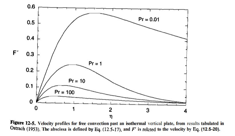
We reproduce figures 12-5 and 12-6 pages 500-501 of textbook Analysis of Transport Phenomena, William M. Deen, Oxford University Press, 1998.
Velocity profiles for the free convection past an isothermal vertical plate
Velocity profiles for the free convection past an isothermal vertical plate
In[]:=
pv=Show[Plot[{f[0.01],f[1],f[10],f[100]},{η,0,5},PlotStyleTable[Hue[i/5],{i,1,4}],Frame->True,GridLines->Automatic,Frame->True,GridLines->Automatic,PlotRange->All,PlotLegends->{Style[0.01,Hue[1/5]],Style[1,Hue[2/5]],Style[10,Hue[3/5]],Style[100,Hue[4/5]]},FrameLabel->{Style["η",14],Style["F'(η)",14]}],ImageSize->400{1,1}]
Digitized data (gray dots) from figures 12-5 of textbook Analysis of Transport Phenomena, William M. Deen, Oxford University Press, 1998.
Temperature profiles for the free convection past an isothermal vertical plate
Temperature profiles for the free convection past an isothermal vertical plate
References
References
1- Simon Ostrach, “An analysis of laminar free - convection flow and heat transfer about a flat plate parallel to the direction of the generating body force”, NACA Tech . Rept . No 1111, pp. 63-79, 1953.
2- William M. Deen, Analysis of Transport Phenomena, Oxford University Press,1998.
CITE THIS NOTEBOOK
CITE THIS NOTEBOOK
Free convection past a vertical flat plate
by Housam Binous and Ahmed Bellagi
Wolfram Community, STAFF PICKS, July 16, 2023
https://community.wolfram.com/groups/-/m/t/2968694
by Housam Binous and Ahmed Bellagi
Wolfram Community, STAFF PICKS, July 16, 2023
https://community.wolfram.com/groups/-/m/t/2968694