Hügelschäffer Egg
Hügelschäffer Egg
A geometric construction of an egg-shaped curve and its surface of revolution
A geometric construction of an egg-shaped curve and its surface of revolution
Summary
Summary
This notebook presents the Hügelschäffer egg, a classical egg-shaped curve obtained from two circles by a simple geometric construction. Starting from the planar curve, we derive its parametric and Cartesian equations and then generate the corresponding three-dimensional egg by rotation about the x-axis.

1. Geometric idea
1. Geometric idea
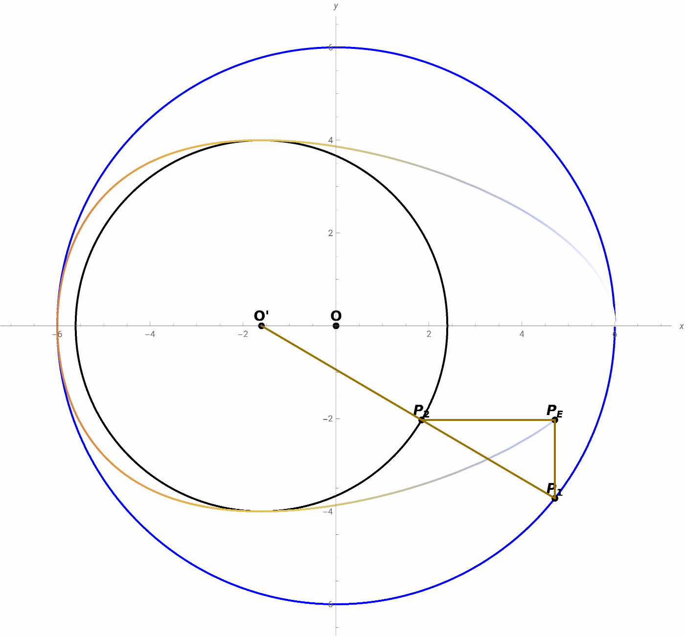
Consider two circles:
◼
a major circle centered at the origin with radius
R
◼
a minor circle centered at with radius r
(d,0)
with .
R > r
A line is drawn from the center of the minor circle, forming an angle θ with the positive x-axis. This line intersects:
(d,0)
◼
the major circle at
P
1
◼
the minor circle at
P
2
The point = (x,y) on the egg curve is obtained by combining:
P
E
◼
the x-coordinate of
P
1
◼
the y-coordinate of
P
2
This produces an asymmetric closed curve with the characteristic shape of an egg.
Reference
Reference
◼
AI-assisted development and personal notes
2. Planar setup
2. Planar setup
We begin with the two circles in parametric form.
ζ[t_]:={RCos[t],RSin[t]}[t_]:={rCos[t]+d,rSin[t]}
ζ
min
A line through and the point on the major circle can be written as:
(d,0)
ζ[t]
{d,0}+w(ζ[t]-{d,0})
which expands to:
{d+w(-d+RCos[t]),RwSin[t]}
3. Intersection with the minor circle
3. Intersection with the minor circle
To locate the intersection with the minor circle, substitute the line into +and solve for w.
2
(x-d)
2
y
2
r
Solve[+==,w]
2
(d+w(-d+RCos[t])-d)
2
(RwSin[t])
2
r
w--2dRdCos[t]++,w-2dRdCos[t]++
r
2
d
2
R
2
Cos[t]
2
R
2
Sin[t]
r
2
d
2
R
2
Cos[t]
2
R
2
Sin[t]
Using the positive branch gives the y-coordinate inherited from the minor-circle intersection. Combining it with the x-coordinate from the major circle yields the egg curve.
4. Parametric equation of the Hügelschäffer egg
4. Parametric equation of the Hügelschäffer egg
P
E
r
2
d
2
R
2
Cos[t]
2
R
2
Sin[t]
This parametrization makes the construction especially transparent:
◼
x(t) = R Cos[t]
◼
y(t)
5. Cartesian equation
5. Cartesian equation
Starting from
Eliminatex==RCos[t],y==R-2dRCos[t]++Sin[t],t//FullSimplify
r
2
d
2
R
2
Cos[t]
2
R
2
Sin[t]
we obtain the Cartesian equation
2
r
2
d
2
R
2
y
or equivalently
2
r
2
R
2
x
2
d
2
R
2
y
This form clearly shows the algebraic relation satisfied by the egg curve.
6. Interactive planar construction
6. Interactive planar construction
In[]:=
ManipulateR=6;r=4;P2[t_]:=d+-2dRCos[t]++(-d+RCos[t]),R-2dRCos[t]++Sin[t];[t_]:=RCos[t],R-2dRCos[t]++Sin[t];ζ[t_]:={RCos[t],RSin[t]};[t_]:={rCos[t]+d,rSin[t]};O1={0,0};O2={d,0};Show[{ParametricPlot[ζ[θ],{θ,0,2π},PlotStyle->{Blue,Thick}],ParametricPlot[[θ],{θ,0,2π},PlotStyle->{Black,Thick}],ParametricPlot[[θ],{θ,0,t},ColorFunction->"BeachColors"],Graphics[{Black,PointSize[0.01],Point[O1],Text[Style["O",14,Bold],O1,{0,-1.2}],Point[O2],Text[Style["O'",14,Bold],O2,{0,-1.2}],Point[ζ[t]],Text[Style["",14,Bold],ζ[t],{0,-1.2}],Point[P2[t]],Text[Style["",14,Bold],P2[t],{0,-1.2}],Point[[t]],Text[Style["",14,Bold],[t],{0,-1.2}],Thick,{DarkYellow,Line[{O2,ζ[t]}],Line[{[t],P2[t]}],Line[{[t],ζ[t]}]}}]},AspectRatioAutomatic,AxesTrue,AxesOrigin{0,0},AxesLabel{x,y},PlotRange{{-6.5,6.5},{-6,6}},ImageSize700],Style["Hügelschäffer Egg",Bold,Large],{{t,0.00002,"Value (t)"},0.000001,2π,0.00001},Delimiter,{{d,-1.60421,"Value (d)"},-2,2,0.00001},ControlPlacementTop
r
2
d
2
R
2
Cos[t]
2
R
2
Sin[t]
r
2
d
2
R
2
Cos[t]
2
R
2
Sin[t]
P
E
r
2
d
2
R
2
Cos[t]
2
R
2
Sin[t]
ζ
min
ζ
min
P
E
P
1
P
2
P
E
P
E
P
E
P
E
P
E
Out[]=


What the animation shows
What the animation shows
7. From curve to solid: a surface of revolution
7. From curve to solid: a surface of revolution
Rotating the planar egg around the x-axis produces a three-dimensional egg-shaped surface.
Interpretation
Interpretation
8. Cartesian equation of the surface of revolution
8. Cartesian equation of the surface of revolution
Starting from
we obtain
This is the Cartesian equation of the three-dimensional egg-shaped surface.
Verification by implicit plotting
Verification by implicit plotting
9. Parametric equation of the surface of revolution
9. Parametric equation of the surface of revolution
Verification by parametric plotting
Verification by parametric plotting
10. Remarks
10. Remarks
The Hügelschäffer egg is a nice example of how a simple geometric prescription can produce:
◼
a visually natural asymmetric curve
◼
an exact parametric representation
◼
an implicit algebraic equation
◼
a convincing three-dimensional egg by revolution
The construction is especially appealing because the geometry, algebra, and visualization reinforce each other.
11. Possible extensions
11. Possible extensions
Some natural directions for further exploration are:
◼
study how the shape changes as d varies
◼
compare the curve with other classical egg curves
◼
examine curvature along the planar profile
◼
compute volume and surface area of the solid of revolution