Product Distribution Curves for Laminar, Plug, and Mixed Flows
Authors: Housam Binous and Ahmed Bellagi
Product Distribution Curves for Laminar, Plug, and Mixed Flows
Authors: Housam Binous and Ahmed Bellagi
Authors: Housam Binous and Ahmed Bellagi
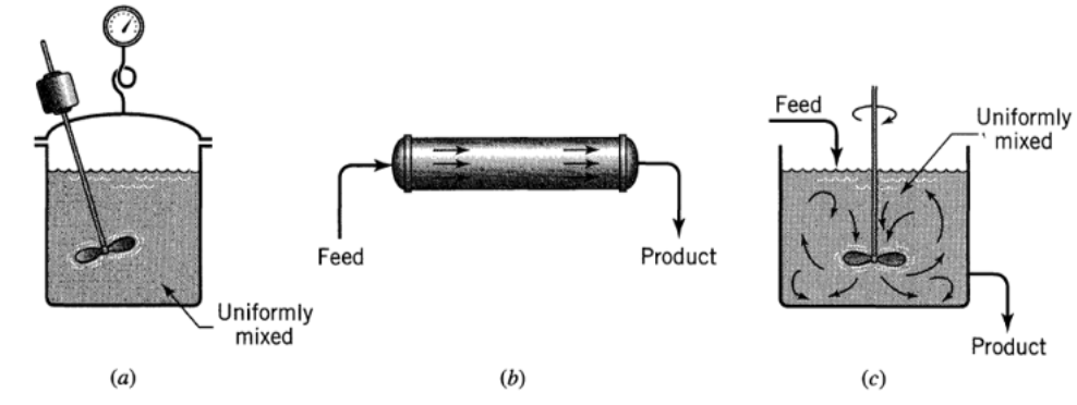
Consider a two-step first-order irreversible reaction in series, A → R → S. We give product distribution curves for the laminar flow (LFR), the plug flow (PFR), and the mixed flow (MFR) reactors. The amount of intermediate formed increases from MFR (green curve) to LFR (blue curve) and finally to PFR (red curve). Deriving expressions for the LFR case is involved (see reference 1).Basic reactor types: (a) Batch, (b) Plug Flow Rector and (c) CSTR or MFR
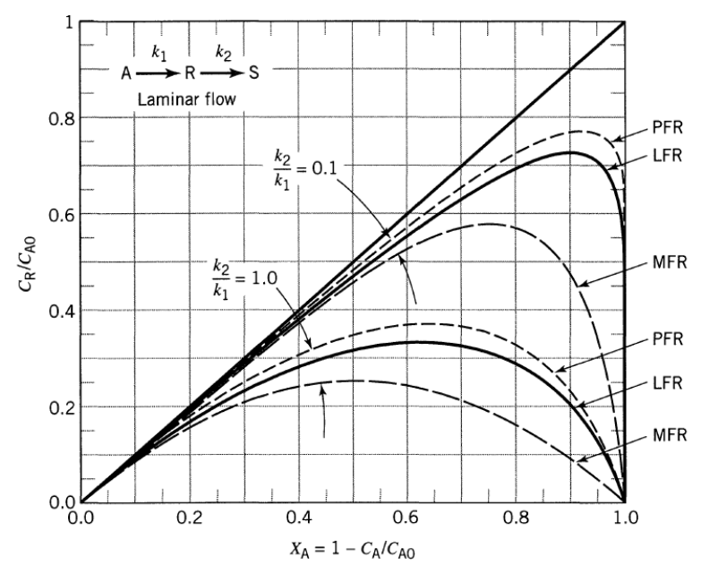
We propose to reproduce a similar figure to Fig. 15-11 page 347 of Textbook by Octave Levenspiel (see reference 2) and given below.
This figure depicts product distribution curves for laminar flow compared with the curves for plug flow and mixed flow.
It indicates that the LFR gives a little less intermediate than does the PFR and significantly more than MFR (about 20 % MORE).
This figure depicts product distribution curves for laminar flow compared with the curves for plug flow and mixed flow.
It indicates that the LFR gives a little less intermediate than does the PFR and significantly more than MFR (about 20 % MORE).
References:
[1] M. M. Johnson, "Correlation of Kinetic Data from Laminar Flow–Tubular Reactors", Industrial & Engineering Chemical Fundamentals, 9(4), 1970 pp. 681–684.
[2] O. Levenspiel, Chemical Reaction Engineering, 3rd ed., New York, NY: Wiley, 1999.
[1] M. M. Johnson, "Correlation of Kinetic Data from Laminar Flow–Tubular Reactors", Industrial & Engineering Chemical Fundamentals, 9(4), 1970 pp. 681–684.
[2] O. Levenspiel, Chemical Reaction Engineering, 3rd ed., New York, NY: Wiley, 1999.
Case 1 : k2/k1=0.1with k1= 2.5; k2 = 0.25;
In[]:=
CA0=1;k1=2.5;k2=0.25;
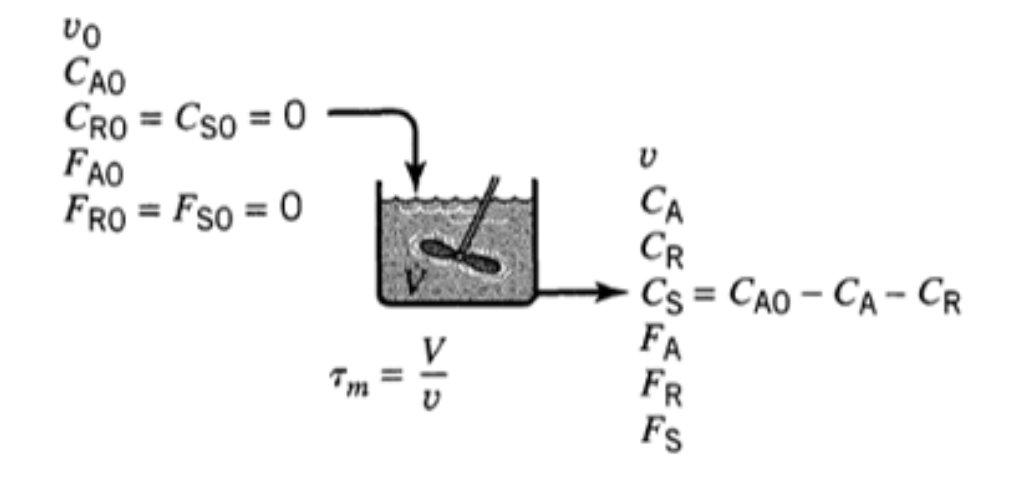
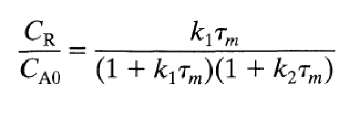
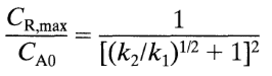
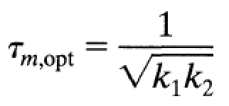
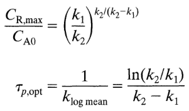
MFRAt steady-state, we have:Position of maximum for intermediate product:if k1=10*k2 we get CA/CA0 = 0.2402 and CR/CA0 = 0.5772
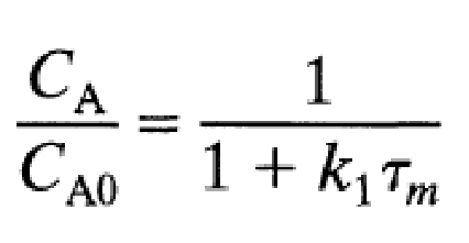
and

In[]:=
data2=Table[{1/(1+k1tau),k1tau/(1+k1tau)/(1+k2tau),1-1/(1+k1tau)-k1tau/(1+k1tau)/(1+k2tau)},{tau,0,50,0.01}];
In[]:=
taumax=1/Sqrt[k1k2]
Out[]=
1.26491
In[]:=
maxMFR={1/(1+k1tau),k1tau/(1+k1tau)/(1+k2tau),1-1/(1+k1tau)-k1tau/(1+k1tau)/(1+k2tau)}/.tau->taumax
Out[]=
{0.240253,0.577215,0.182532}
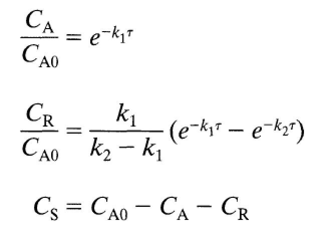
PFRThe above expression are identical to what one would get for a Batch reactor except that we replace time, , with residence time τ.Position of maximum for intermediate product:if k1=10*k2 we get CA/CA0 = 0.0774 and CR/CA0 = 0.7742
t
LFR
Ternary plot with product distribution for MFR, PFR and LFR
Digitized data of Fig. 15-11 page 347 of Textbook by Octave Levenspiel (see reference 2)
Digitized data put in proper format
Our results for MFR, PFR and LFR agree with their counterparts obtained by digitizing Fig. 15-11 page 347 of Textbook by Octave Levenspiel (see reference 2)
BLACK DOTS represent the loci of the optimum intermediate product
BLACK DOTS represent the loci of the optimum intermediate product
MFR
Position of maximum for intermediate product:
if k1=k2 we get CA/CA0 = 0.50 and CR/CA0 = 0.25
Position of maximum for intermediate product:
if k1=k2 we get CA/CA0 = 0.50 and CR/CA0 = 0.25
PFR
Position of maximum for intermediate product:
if k1=k2 we get CA/CA0 = 0.3678 and CR/CA0 = 0.3678
Position of maximum for intermediate product:
if k1=k2 we get CA/CA0 = 0.3678 and CR/CA0 = 0.3678
LFR
Ternary plot with product distribution for MFR, PFR and LFR
Digitized data of Fig. 15-11 page 347 of Textbook by Octave Levenspiel (see reference 2)
Digitized data put in proper format
Our results for MFR, PFR and LFR agree with their counterparts obtained by digitizing Fig. 15-11 page 347 of Textbook by Octave Levenspiel (see reference 2)
BLACK DOTS represent the loci of the optimum intermediate product
BLACK DOTS represent the loci of the optimum intermediate product
We propose to reproduce Fig. 8-6 page 178 of Textbook by Octave Levenspiel (see reference 2) and given below.
This figure depicts a comparison of the fractional yields of R in mixed flow and plug flow reactors for a two-step first-order irreversible reaction in series:
A → R → S
This figure depicts a comparison of the fractional yields of R in mixed flow and plug flow reactors for a two-step first-order irreversible reaction in series:
A → R → S
This figure depicts a comparison of the fractional yields of R in mixed flow and plug flow reactors for a two - step first - order irreversible reaction in series :
A → R → S.
Coloured solid lines (our calculation) and gray dots (digitized data of Levenspiel’s textbook).
A → R → S.
Coloured solid lines (our calculation) and gray dots (digitized data of Levenspiel’s textbook).