Supercharge your optimization problem solving with Gurobi
Supercharge your optimization problem solving with Gurobi


The Wolfram Language provides a that solve optimization problems: It can solve symbolic and numerical optimization problems, local and global problems, linear and nonlinear problems, and convex and non-convex optimization problems. Each type of optimization problem has its own solution algorithms and the Wolfram Language makes it easy to use all of them thanks to a well-designed top-level interface and built-in automatic algorithm selection.
But solving optimization problems quickly is a complex algorithmic challenge: There are no “provably fastest” algorithms in this field. Many new state-of-the-art algorithms are discovered every year, pushing the performance boundary farther and farther. To give Wolfram Language access to these bleeding edge solvers we developed a general optimization framework which allows you to leverage any number of them.
To make things even easier for numerical problems, Wolfram Research provides built-in support for a state-of-the-art solver from Gurobi, a company with a singular focus on providing the fastest optimization solver in the world. Their flagship product, the Gurobi Optimizer, is significantly faster than other solvers and solves the following major optimization types (including real-valued and mixed-integer sub-types): Linear Optimization, Quadratic Optimization, Second-Order Cone Optimization, and Quadratically Constrained Optimization.
In this post I will give a gentle introduction into what is possible with the Gurobi Optimizer and how you can use the Wolfram Language to specify optimization problems at a very high level, with its built-in typesetting capabilities, its first-class symbolic preprocessing functions, and its out-of-this-world visualization features.
First, let’s take a look at how the Gurobi-supported optimization types and their abbreviations map into Wolfram Language functions:
Optimization type | Wolfram Language function |
(Mixed-Integer) Linear Optimization | |
(Mixed-Integer) Quadratic Optimization | |
(Mixed-Integer) Second-Order Cone Optimization | |
(Mixed-Integer) Quadratically Constrained Optimization |
The Basics — Linear Optimization
The Basics — Linear Optimization
Let’s start by looking at a very simple linear optimization problem, where both the cost function and the constraints are linear functions with any number of decision variables:
Minimize: Subject to:
2x+3y
3x+6y>=25
y>=-3x+9
x>=0,y>=0
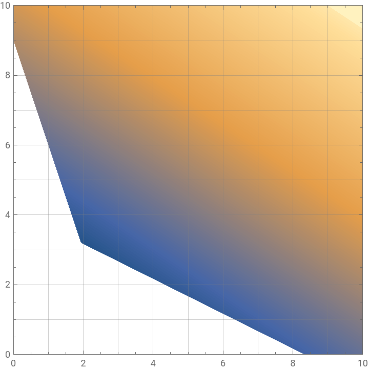
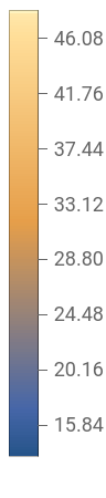
In this simple case with two decision variables (x and y), we can visualize feasible region with a ContourPlot. Here, the orange-blue shading represents the values of the cost function (irrelevant plotting details and options have been elided (…) with the iconize feature of the Wolfram Notebook interface):
ContourPlot2x+3y,{x,0,10},{y,0,10},RegionFunction->Function[{x,y},x>=0&&y>=0&&3x+6y>=25&&y>=-3x+9],
We now use the LinearOptimization function to get an answer, and specify the result types we’re interested in (in this case the primal minimum value and the primal minimizer values). To use the Gurobi Optimizer, we set the Method option to "Gurobi":
{minimum1,minimizer1}=LinearOptimization[2x+3y,{x>=0,y>=0,3x+6y>=25,y>=-3x+9},{x,y},{"PrimalMinimumValue","PrimalMinimizer"},
Method"Gurobi"
]{13.4667,{1.93333,3.2}}
It is easy to change this problem into a mixed-integer problem by specifying the types of the variables:
{minimum2,minimizer2}=LinearOptimization[2x+3y,{x>=0,y>=0,3x+6y>=25,y>=-3x+9},
{x∈Integers,y∈Reals}
,
{"PrimalMinimumValue","PrimalMinimizer"},Method"Gurobi"]{13.5,{2,3.16667}}
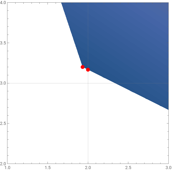
We use a ContourPlot to zoom in on the location of both solutions
ContourPlot2x+3y,{x,0,10},{y,0,10},RegionFunction->Function[{x,y},x>=0&&y>=0&&3x+6y>=25&&y>=-3x+9],Epilog{Red,AbsolutePointSize[8],
Point[{minimizer1,minimizer2}]
},
The need for speed…
The need for speed…
For simple optimization problems the built-in solver has about the same performance as the Gurobi Optimizer: you get the same result and both solvers return the answer in the blink of an eye. But most real-world optimization problems have large numbers of variables and constraints. To show the difference in performance between the built-in solver (CLP) and the Gurobi Optimization we can create an example with a SparseArray. The SolverTiming function below accepts a size argument (“n”) and a solver method (“Gurobi” or “CLP”)
SolverTiming[n_,method_]:=Module[{c,a,b},c=ConstantArray[1.0,n];a=SparseArray[{Band[{1,1}]->2.0,Band[{2,1}]->ConstantArray[1.0,n-1],Band[{1,2}]->1.0,Band[{n+1,1}]->1.0},{2n,n}];b=Join[ConstantArray[-100.0,n],ConstantArray[0.,n]];First[AbsoluteTiming[
LinearOptimization[c,{a,b},Method->method]
]]]We can now use the SolverTiming function to create a dataset table for increasing problem sizes and their timings for each solver:
ds=Dataset[Table[<|"Size"n,"Gurobi"SolverTiming[n,"Gurobi"],"CLP"SolverTiming[n,"CLP"]|>,{n,10000,50000,5000}]]
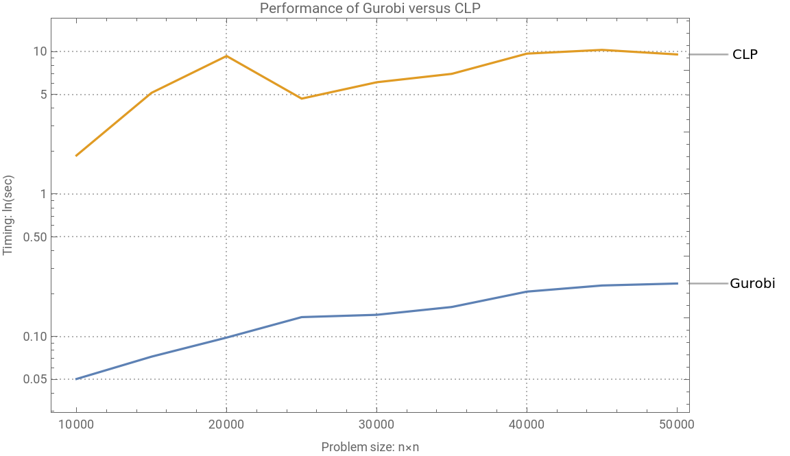
And we can compare the performance in a ListLogPlot, showing that Gurobi is more than an order of magnitude faster than the CLP solver for this particular problem:
data=Values@Normal@ds;ListLogPlot{data[[All,{1,2}]],data[[All,{1,3}]]},
Note that I am using a very simple linear optimization example here. The Gurobi Optimizer excels in many areas, especially in mixed-integer problems. For more in-depth information on its performance, please visit Gurobi's Benchmarking web page.
Importing optimization problems…
Importing optimization problems…
Quadratic Optimization
Quadratic Optimization
Now let’s take a look at a few quadratic optimization problems that you can solve with the Gurobi Optimizer. The QuadraticOptimization function can solve both real and mixed-integer problems.
One nice feature of the Wolfram Language is that you can use use common compact matrix and vector notation to specify your problem. Here we randomly generate the problem parameters and use vector inequality () for notation:
And get the solution using the Gurobi Optimizer:
If we want to change this to a pure integer quadratic optimization problem, we can simply change the vector type:
Or we can create a mixed-integer problem. This example has 3 real decision variables and 5 integer decision variables:
Using high-level Wolfram Language functions…
Using high-level Wolfram Language functions…
Another nice feature of Wolfram Language’s optimization framework is the ability to translate a higher-level symbolic problem formulation into a form that the Gurobi Optimizer can process. An example of this can be seen with this example where we use Total[…] to compactly represent the sum of the elements of the vector x and Norm[…] as the square root of the sum of the squares of the elements.
There are many higher-level Wolfram Language functions that you can use on vectors and matrices, including all basic arithmetic functions and distance functions.
This is equivalent to writing the following statement:
Other region-based primitives include polygons and polyhedrons.
The best of both worlds…
The best of both worlds…
The documentation pages for LinearOptimization, QuadraticOptimization, SecondOrderConeOptimization, and ConvexOptimization contain hundreds of interesting application examples which make it very easy to get started on using the Wolfram Language with the Gurobi Optimizer: From inventory control problems, manufacturing problems, and transportation problems, to solving mathematical puzzles like Sudoku, the travelling salesman problem, and portfolio optimization.
For highly technical people, and especially those well-versed in the Wolfram, we have also recently open-sourced our implementation which shows how the connection from the Wolfram Language to the Gurobi Optimizer works “under the hood”. It is named GurobiLink, and is located on the Wolfram Research Github page.
Working with the Gurobi Optimizer in the Wolfram Language gives you the best of both worlds: Leading solver performance for optimization problems coupled with the world’s best computational language for scientific and business applications.
To learn more about Gurobi and how tot get the Gurobi Optimizer, visit: https://www.gurobi.com/
To learn more about Wolfram Research and the Wolfram Language, visit: https://www.wolfram.com/