We explore continuous cellular automata, by investigating different neighborhood sizes and activation functions, and see how small perturbations affect their evolution. We classify the resulting automata according to their complexity. We investigate intrinsic randomness generation and sensitivity to initial conditions, while on the way toward building a computational tool, for studying the foundation of chaotic string theory, using Wolfram Mathematica.
Introduction
Introduction
Notes
Notes
The code in each of the three sections below needs to be run separately, by restarting the kernel.
Throughout this essay, we perform the main computations with accuracy set to : .
4
10
N_,∞,
4
10
Sometimes the Manipulate function may simply be needing more time to evaluate, despite an “$Aborted” message.
If it does really abort at the beginning, simply adjust and then re-adjust a parameter.
An external reference is indicated in bold by a number within square brackets. For example, [4] means reference 4.
A reference within this essay is indicated by a number and character(s) separated by hyphen(s) within parentheses. For example, (2-d-D) means Section 2, Subsection d, Subsubsection D.
Motivation
Motivation
In this computational essay, we do some fundamental exploration in what are called continuous cellular automata, sometimes also known as coupled map lattices. Basically, these are just cellular automata, with each cell containing a value from a continuous range of real numbers.
Some special types of these systems are known as chaotic strings, which have been used to correctly predict several fundamental parameters of physics [2, 5, 6], following the approach taken in [1], but using chaotic noise instead of white noise.
In [7], I have written a program in Wolfram Mathematica aimed at validating the prediction of one of the parameters, namely the electric fine structure “constant” at the energy scale of 3 times the mass of an electron, shown on pp. 11-12 in [2] and on pp. 133-136 in [5].
The main motivation for the current exploration comes from the following two sources:
(A) In [3], the following two challenges have been raised regarding chaotic string theory [2, 5, 6]:
(a1) If chaotic noise is what is needed in order to simulate quantum noise, why do most of the physically relevant values of the coupling parameter correspond to stability rather than chaos?
(a2) For making the correct physical predictions, why does it seem necessary to start with only certain special initial conditions? Does this mean that the predictions are actually somehow already coded in the initial conditions themselves?
(B) In [4], on pp. 149-155, the following crucial observations have been made:
(b1) A number’s digit sequence can sometimes be at least as important as its size.
(b2) The iterations of some functions converge to some uniform pattern, independent of the initial conditions.
(b3) The iterations of some functions simply display the randomness or complexity inherent in the initial conditions. They do not generate randomness or complexity if the initial conditions are simple.
(b4) However, there are some functions whose iterations can generate intrinsic randomness or complexity, independent of the initial conditions.
The eventual goal of the present work is to make progress toward answering (a1-2) above by using (b1-4) above.
Here we do some basic studies about how small perturbations affect the evolution of various continuous cellular automata.
We will continue to address the above questions (a1-2) in more detail in a future work.
Overview
Overview
Section 1 (Various types of effect of small perturbations)
Section 1 (Various types of effect of small perturbations)
In Section 1, we do some basic studies of continuous cellular automata, by categorizing the various types of patterns generated when subtracting a small value δ from the initial value 1, where δ is a small perturbation within the range .
Range0,,
1
100
1
100000
Section 2 (Intrinsic randomness generation and sensitivity to initial conditions)
Section 2 (Intrinsic randomness generation and sensitivity to initial conditions)
In Section 2, we investigate how the overall evolution changes when we:
(A) perturb the initial conditions very slightly by adding a tiny perturbation δ = , and also
-20
10
(B) change the initial conditions themselves between having a simple digit sequence and having a complicated digit sequence.
By starting with the number which has a simple digit sequence, and with the number which has a complicated digit sequence, and by using the 4 different mappings as shown on p. 150 of [4], we explore the phenomena of intrinsic randomness generation and sensitivity to initial conditions.
1
2
π
6
When starting with the number , if we see an apparently random behavior which is qualitatively similar to the behavior when starting with the number ,then we know that the behavior is independent of the complexity of the digit sequence of the initial conditions.This means that the apparent randomness is not coming from the initial conditions.Therefore, we have intrinsic randomness generation.
1
2
π
6
Starting with a tiny perturbation δ, as the iteration proceeds, if large differences suddenly start arising after some point,
then we say that there is sensitivity to initial conditions.
then we say that there is sensitivity to initial conditions.
Comparing with what has been observed on pp. 150-151 in [4]:
Case (a): Here also, we observe both intrinsic randomness generation and sensitivity to initial conditions.
Case (b): Again, we observe both intrinsic randomness generation and sensitivity to initial conditions.
Case (c): Here also, we observe evolution to zero, independent of the initial conditions.
Case (d): Here, we do observe sensitivity to initial conditions. However, unlike what has been observed for case (d) on pp. 150-151 in [4], here in the case of continuous cellular automata, we observe intrinsic randomness generation for this case, as we see below in (2-d-D).
Section 3 (Chaotic Strings)
Section 3 (Chaotic Strings)
In Section 3, we extend the investigation of Section 2 to chaotic strings.
We investigate with the total of 26 special values of the parameter a listed in Tables 12.1-3 on pp. 241-244 in [5] and in Tables 1-3 on pp. 20-23 in [6].
Corresponding to each value of a, we consider three values -- including the slightly lower value and the slightly higher value based on the given uncertainty.
Therefore, we compute a total of 26 × 3 = 78 cases -- each of these cases further splitting into two -- one corresponding to the initial value , and the other corresponding to the initial value .
1
2
π
6
We discover that all these results show both intrinsic randomness generation and sensitivity to initial conditions.
(1) Various types of effect of small perturbations
(1) Various types of effect of small perturbations
First, we make sure to exit any previous kernel session:
In[]:=
Exit[]
(a) Introduction
(a) Introduction
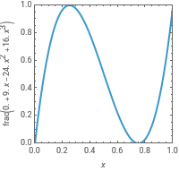
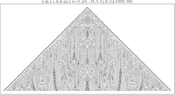
We define a customizable activation function, and study the cellular automaton evolution for neighborhood radius = 1, 2 and 3.
In this section the way we use the activation function is the following:
Algorithm 1:
(A) Corresponding to each cell, take the average of all the cells in its neighborhood, and apply the activation function to the average. The result is the new value of the cell on the next row.
(B) After computing the values of all the cells in the new row, subtract the average of the neighboring cells from the value of each cell, and take the absolute value of the result. This helps to filter out some stripe patterns.
The initial value is (1 - δ), where δ is a small perturbation within the range .
Range0,,
1
100
1
100000
By varying the value of δ, we observe whether there is any change in the overall pattern.
We examine the effects of small perturbations to the simple initial conditions, and gather the results into the following three groups, and then, within each group, classify further into Classes 1, 2, 3 and 4, as applicable:
(1-d) Results stable with respect to small perturbations
(1-e) Results sensitive with respect to small perturbations
(1-f) Results sensitive only at particular threshold values of perturbation
(b) Main code
(b) Main code
(c) Experiments
(c) Experiments
Manipulate
Manipulate
Out[]=


Sample code for specific cases
Sample code for specific cases
(d) Results stable with respect to small perturbations
(d) Results stable with respect to small perturbations
In these cases, categorized into Classes 1-4, changes within the used range of δ-values do not seem to affect the cellular automaton evolution:
Class 1
Class 1
Class 2
Class 2
Class 3
Class 3
Class 4
Class 4
(e) Results sensitive with respect to small perturbations
(e) Results sensitive with respect to small perturbations
In these cases, categorized into Classes 1-4, changes within the used range of δ-values do seem to affect the cellular automaton evolution:
Class 1
Class 1
Class 2
Class 2
Class 3
Class 3
Class 4
Class 4
(f) Results sensitive only at particular threshold values of perturbation
(f) Results sensitive only at particular threshold values of perturbation
In these cases, categorized into Classes 1-4, changes within the used range of δ-values seem to affect the cellular automaton evolution, but for each case at only a certain threshold value of δ:
Class 1
Class 1
Class 2
Class 2
Class 3
Class 3
Class 4
Class 4
(2) Intrinsic randomness generation and sensitivity to initial conditions
(2) Intrinsic randomness generation and sensitivity to initial conditions
First, we exit the kernel, in order to restart it for this new section:
(a) Introduction
(a) Introduction
In this section also, we similarly define a customizable activation function, and study the cellular automaton evolution for neighborhood radius = 1, 2 and 3.
Here, the way we use this activation function is the following:
Algorithm 2:
(A) Corresponding to each cell, take the average of all the cells in its neighborhood, and apply the activation function to the average. The result is the new value of the cell on the next row.
For the initial values, we first use an initial value u, where u is a number, either rational or irrational.
Next, we use the initial value (u + δ), where δ is a small perturbation.
We compute and study the behavior of the absolute values of the differences between the above two results as the cellular automaton evolution proceeds.
Corresponding to each row, we take the average of the above absolute values and plot it as a function of the iteration number.
(c) Experiments
(c) Experiments
(d) Results
(d) Results
A
A
B
B
C
C
D
D
(3) Chaotic Strings
(3) Chaotic Strings
Again, we exit the kernel, in order to restart it for this new section:
(a) Introduction
(a) Introduction
We investigate intrinsic randomness generation and sensitivity to initial conditions in the case of the eight (based on the values of n, b and s) continuous cellular automata (the so-called chaotic strings), for various values of the coupling parameter a, as indicated below, for a radius-1 neighborhood.
n ∈ {2, 3}
b ∈ {1, 0}
s ∈ {+1, -1}
0 ≤ a ≤ 1
b ∈ {1, 0}
s ∈ {+1, -1}
0 ≤ a ≤ 1
Corresponding to the different values of n, b and s, we obtain the following 8 different chaotic strings:
We investigate with the total of 26 special values of the parameter a listed in Tables 12.1-3 on pp. 241-244 in [5] and in Tables 1-3 on pp. 20-23 in [6].
As mentioned near the beginning of this essay, the results below in this section should help towards addressing the concerns expressed in [3], regarding the foundation of the theory of chaotic strings [2, 5, 6].
(c) Experiments
(c) Experiments
Since we work in the domain [-1, +1] in this section, we use the following color code:
(d) Results
(d) Results
Here are some useful definitions used to compute and collect the main results below for this section:
Now we are ready to compute and collect the main results:
Concluding Remarks
Concluding Remarks
When exploring several continuous cellular automata, including chaotic strings, we have found both intrinsic randomness generation and sensitivity to initial conditions.
This foundational work will help to examine and strengthen the foundation of chaotic string theory which correctly predicts various physical parameters of fundamental physics.
We will continue more detailed investigations in a future work.
Acknowledgments
Acknowledgments
It has been my good fortune to have, as my mentor for this project, Dugan Hammock who has been very kind, helpful and supportive.
Dugan’s amazingly acute observation, of visually almost indistinguishable asymmetry in some of the cellular automata plots, opened my eyes to the risk involved in working with machine precision, and hence was crucial in setting the direction of my research.
From the very beginning, I have been grateful to Xerxes Arsiwalla for his enthusiastic encouragement, high-level support and wise guidance throughout my research.
I greatly appreciate Stephen Wolfram for kindly, and with deep understanding and foresight, suggesting to me this project which is foundational for my longer-term research goals.
From the bottom of my heart, I thank Stephen and the entire Wolfram Summer School 2025 team for organizing this wonderful program, which is a very enjoyable and special experience in my life.
Thank you!!
References
References
1
.Giorgio Parisi and Yongshi Wu (1981), “Perturbation theory without gauge fixing”, Scientia Sinica, Volume XXIV, Number 4.
https://dds.sciengine.com/cfs/files/pdfs/view/1000-0002/ND788HY5Zy6xPfrcr.pdf
https://dds.sciengine.com/cfs/files/pdfs/view/1000-0002/ND788HY5Zy6xPfrcr.pdf
2
.Christian Beck (2001), “Chaotic strings and standard model parameters”, arXiv.
https://arxiv.org/pdf/hep-th/0105152
https://arxiv.org/pdf/hep-th/0105152
3
.Carl P Dettmann (2002), “Stable synchronised states of coupled Tchebyscheff maps”, Physica D: Nonlinear Phenomena, Volume 172, Issue 1-4.
https://arxiv.org/pdf/nlin/0110007
https://arxiv.org/pdf/nlin/0110007
4
.Stephen Wolfram (2002), A New Kind Of Science. Wolfram Media, Inc.
https://www.wolframscience.com/nks/
https://www.wolframscience.com/nks/
5
.Christian Beck (2002), Spatio Temporal Chaos and Vacuum Fluctuations of Quantized Fields. World Scientific Publishing Co. Pte. Ltd.
https://www.amazon.com/Spatio-Temporal-Vacuum-Fluctuations-Quantized/dp/9810247982
https://www.amazon.com/Spatio-Temporal-Vacuum-Fluctuations-Quantized/dp/9810247982
6
.Christian Beck (2002), “Spatio-temporal Chaos and Vacuum Fluctuations of Quantized Fields”, arXiv.
https://arxiv.org/pdf/hep-th/0207081
https://arxiv.org/pdf/hep-th/0207081
7
.Cite This Notebook
Cite This Notebook
Exploring continuous cellular automata with respect to small perturbations
by Kiran Shrestha
Wolfram Community, September 12, 2025
https://community.wolfram.com/groups/-/m/t/3497743
by Kiran Shrestha
Wolfram Community, September 12, 2025
https://community.wolfram.com/groups/-/m/t/3497743